University of Florida/Egm4313/IEA-f13-team10/R2

Problem Statement

Show the equivalence between the two statements that define the linearity of differential operators.

Statement (1):
The definition of a linear operator, ${\displaystyle {\mathcal {D}}}$, is

${\displaystyle {\mathcal {D}}(cy+kw)=c{\mathcal {D}}(y)+k{\mathcal {D}}(w)}$

for any two constants ${\displaystyle c}$ and ${\displaystyle k}$, and for any two functions ${\displaystyle y(.)}$ and ${\displaystyle w(.)}$

Statement (2):
The operator ${\displaystyle {\mathcal {D}}}$ is linear iff

${\displaystyle {\mathcal {D}}(\alpha y)=\alpha {\mathcal {D}}(y)}$
for any constant ${\displaystyle \alpha }$ and for any function ${\displaystyle y(.)}$,

and

${\displaystyle {\mathcal {D}}(y+w)={\mathcal {D}}(y)+{\mathcal {D}}(w)}$
for any two functions ${\displaystyle y(.)}$ and ${\displaystyle w(.)}$.

Solution

We saw on piazza how to prove statement (1) from statement (2). To prove statement (2) from statement (1) we choose clever values for the constants ${\displaystyle c}$ and ${\displaystyle k}$ and for the functions ${\displaystyle y(.)}$ and ${\displaystyle w(.)}$.

Honor Pledge

On our honor, we solved this problem on our own, without aid from online solutions or solutions from previous semesters.

Problem Statement

Build on my note in the same piazza post on differential operators on the notation ${\displaystyle {\mathcal {D}}}$
for general differential operators, and the notation ${\displaystyle D}$
as defined in Eq.(1) in K 2011, sec.2.3, to explain the similarities and differences between these two notations.

Solution

The similarity with both ${\displaystyle {\mathcal {D}}}$ and ${\displaystyle D}$ is that they look like they're both upper case D's. Both of these D's also symbolized the differential operator.
The difference between both of these D's is that ${\displaystyle {\mathcal {D}}}$
is a generalized differential operator, which can be seen as ${\displaystyle {\mathcal {D}}=d^{n}/dx^{n}}$
and ${\displaystyle D}$ refers to the first differential operator: ${\displaystyle D={d \over dx}}$

Honor Pledge

On our honor, we solved this problem on our own, without aid from online solutions or solutions from previous semesters.

Problem Statement

${\displaystyle y''+8y'+15y=\sin x}$

${\displaystyle y(0)=1,\ y'(0)=0}$

Identify the polynomial ${\displaystyle P(D)}$ as defined in K 2011, sec.2.3, for this problem.
Then rewrite the above problem in terms of the linear differential operator ${\displaystyle L=P(D)}$.
Use its linear property to demonstrate the above problem into a homogeneous part and a particular part.
How would the initial conditions be written in terms of the homogeneous solution and the particular solution?

Solution

${\displaystyle L=P(D)=D^{2}+8D+15}$
${\displaystyle L(y)=sin(x)}$
Let ${\displaystyle y=y_{h}+y_{p}}$
${\displaystyle L(y_{h}+y_{p})=sin(x)}$
${\displaystyle L(y_{h})+L(y_{p})=sin(x)}$

Splitting into homogeneous and particular,
${\displaystyle L(y_{h})=0}$
${\displaystyle L(y_{p})=sin(x)}$

Inputting the initial conditions,
${\displaystyle y(0)=1=y_{h}(0)+y_{p}(0)}$
${\displaystyle y'(0)=0=y_{h}'(0)+y_{p}'(0)}$

Honor Pledge

On our honor, we solved this problem on our own, without aid from online solutions or solutions from previous semesters.

Problem Statement

Given the two roots an the initial conditions:
${\displaystyle \lambda _{1}=-2,\lambda _{2}=5}$
${\displaystyle y(0)=1,y'(0)=0}$

Find the non-homogeneous L2-ODE-CC in standard form
and the solution in terms of the initial conditions
and the general excitation ${\displaystyle r(x)}$.
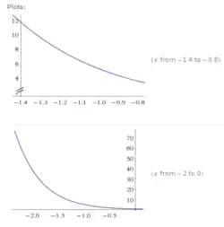
Consider no excitation
${\displaystyle r(x)=0}$
Plot the solution

Solution

${\displaystyle (r+2)(r-5)=0}$
${\displaystyle r^{2}-3r-10=0}$
${\displaystyle \lambda ^{2}-3\lambda -10=0}$
${\displaystyle y''+3y'-10y=r(x)}$

${\displaystyle y_{h}(x)=c_{1}e^{-2x}+c_{2}e^{5x}+y_{p}(x)}$
${\displaystyle y_{p}(x)=r(x)=0}$
Therefore, ${\displaystyle y_{h}(x)=c_{1}e^{-2x}+c_{2}e^{5x}}$
${\displaystyle y'_{h}(x)=-2c_{1}e^{-2x}+5c_{2}e^{5x}}$

Solve for constants ${\displaystyle c_{1}}$ and ${\displaystyle c_{2}}$:
${\displaystyle y(0)=1=c_{1}+c_{2}}$
${\displaystyle y(0)=0=-2c_{1}+5c_{2}}$

${\displaystyle c_{1}=1-c_{2}}$
${\displaystyle -2(1-c_{2})+5c_{2}=0}$
${\displaystyle -2+2c_{2}+5c_{2}=0}$
${\displaystyle 7c_{2}=2}$

${\displaystyle c_{2}=2/7}$
${\displaystyle c_{1}=5/7}$
so,
${\displaystyle y(x)=5/7e^{-2x}+2/7e^{5x}}$

Honor Pledge

On our honor, we solved this problem on our own, without aid from online solutions or solutions from previous semesters.

Problem Statement

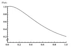
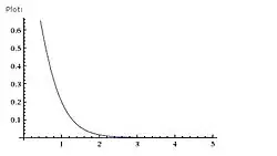
Find the general solution to the ODE ${\displaystyle y''+2\pi y'+\pi ^{2}y=0}$
With the initial values y(0) = 1 and y'(0) = .5

Solution

${\displaystyle y''+2\pi y'+\pi ^{2}y=0}$

This is a linear, first order ODE with constant coefficients.

To find the general solution to this ODE set ${\displaystyle y=e^{rx}}$

so that ${\displaystyle y'=re^{rx}}$ and ${\displaystyle y''=r^{2}e^{rx}}$

Substituting in y to the ODE and factoring out ${\displaystyle e^{rx}}$ we get:

${\displaystyle r^{2}+2\pi r+\pi ^{2}=0}$

Using the quadratic formula to solve for r we get

${\displaystyle r={\frac {-b\pm {\sqrt {b^{2}-4ac}}}{2a}}}$ where ${\displaystyle a=1,b=2\pi ,}$ and ${\displaystyle c=\pi ^{2}}$

Solving to get ${\displaystyle r=-\pi }$

Since we have a repeated root, we need to find v(x) so that y2(x) = v(x)y1(x)

Taking the first and second derivative of y2(x) we get:

${\displaystyle y_{2}'(x)=v'(x)y_{1}(x)+v(x)y_{1}'(x)}$
${\displaystyle y_{2}''(x)=v''(x)y_{1}(x)+2v'(x)y_{1}(x)+v(x)y_{1}''(x)}$

solving for ${\displaystyle v''(x)=0}$ so ${\displaystyle v(x)=kx+c}$

So y2(x) = x y1(x)

We get the general solution ${\displaystyle y(x)=C_{1}e^{-\pi x}+C_{2}xe^{-\pi x}}$

Now with the initial values y(0) = 1 and y'(0) = .5

${\displaystyle y(0)=C_{1}=1}$

${\displaystyle y'(0)=-\pi C_{1}+C_{2}=.5}$

${\displaystyle C_{1}=1}$ , ${\displaystyle C_{2}=3.64}$

${\displaystyle y(x)=e^{-\pi x}+3.64xe^{-\pi x}}$

${\displaystyle 0<x<1}$ ${\displaystyle 0<x<5}$

Honor Pledge

On our honor, we solved this problem on our own, without aid from online solutions or solutions from previous semesters.

Problem Statement

Discuss the similarities and differences between Coulomb friction / damping (piazza post) with the damper used in the SDOF spring-mass-damper system with 2 ends fixed.

Solution

Honor Pledge

On our honor, we solved this problem on our own, without aid from online solutions or solutions from previous semesters.