University of Florida/Egm4313/IEA-f13-team10/R3
Report 3
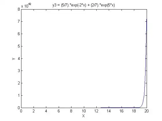
Problem 1
Problem Statement
Find the complete homogeneous solution using variation of parameters

Solution
The solution is
Therefore, and
Plugging this back into the original homogeneous equation,
so


Checking the answer


Plugging this into the original homogeneous equation

Plugging in values for y and its derivatives, everything cancels out to zero.
Honor Pledge
On our honor, we solved this problem on our own, without aid from online solutions or solutions from previous semesters.
Problem 2
Problem Statement
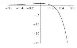
Find and plot the solution for the L2-ODE_CC


Solution
This is a linear, first order ODE with constant coefficients.

To find the general solution to this ODE set
so that and
Substituting in y to the ODE and factoring out we get:


Using the quadratic formula to solve for r we get
where and


Solving to get

Since we have a repeated root, we need to find v(x) so that y2(x) = v(x)y1(x)
Taking the first and second derivative of y2(x) we get:


Substituting into the original ODE, we get:
solving for so v(x) = kx + c


So y2(x) = x y1(x)
We get the general solution

Now with the initial values y(0) = 1 and y'(0) = 0


,


Honor Pledge
On our honor, we solved this problem on our own, without aid from online solutions or solutions from previous semesters.
Problem 3
Problem Statement
Problem Sec 2.4 problem 3
How does the frequency of the harmonic oscillation change if we (i) double the mass (ii) take a spring of twice the modulus?
Problem Sec 2.4 problem 4
Could you make a harmonic oscillation move faster by giving the body a greater push?
Solution
Problem Sec 2.4 problem 3
Part 1
Now double the mass
The frequency is decreased by .


Part 2
Multiply k by 2
The frequency is increased by .

Problem Sec 2.4 problem 4
No because frequency depends on the ratio of the spring modulus and mass.
Honor Pledge
On our honor, we solved this problem on our own, without aid from online solutions or solutions from previous semesters.
Problem 4
Problem Statement
Section 2.4 Problem 16
Show the maxima of an underdamped motion occur at equidistant t-values and find the distance.
Section 2.4 Problem 17
Determine the values of t corresponding to the maxima and minima of the oscillation . Check your result by graphing y(t).

Solution
Section 2.4 Problem 16
Part 1=
The general solution of underdamped motion is
The maximas occur at
Set the two equations equal to each other a solve for t.
where n=0,1,2,3.....


Part 2
shows delta is a constant.
The periodic distance between maximas is


Section 2.4 Problem 17
To find critical points, set y'(t)=0
![{\displaystyle y'(t)=e^{-t}[-sin(t)+cos(t)]}](../../../../I/91534de525e96b17fce3b759cacea5a8ae9bbfaf.svg)
where n=0,1,2,3...
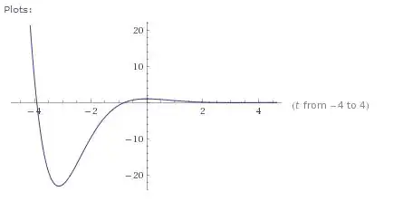
As seen in the graph, the maximum of t was at and the minimum was at .
![{\displaystyle e^{-t}[-sin(t)+cos(t)]=0}](../../../../I/b2d768e780794f3e0303c59eaea39f394619d8da.svg)
![{\displaystyle [-sin(t)+cos(t)]=0}](../../../../I/f4b4d0b351c4305b7abe9fde6305c1397dfcb422.svg)


Honor Pledge
On our honor, we solved this problem on our own, without aid from online solutions or solutions from previous semesters.
Problem 5
Problem Statement
Using the formula for Taylor series at x = 0 (the origin, i.e., McLaurin series), develop into Taylor series at the origin x = 0 for the following functions: cos x, sin x, exp(x), tan x, and write these series in compact form with the summation sign and a single summand.
Solution
Part 1
cos x
Taylor Series:
when


n = 0, 1, 2, 3 ... N
2n = 0, 2, 4, 6, ... 2N

Part 2
sin x
Taylor Series:
when


Part 3
exp x
Taylor Series:
when


Honor Pledge
On our honor, we solved this problem on our own, without aid from online solutions or solutions from previous semesters.
Problem 6
Problem Statement
Part 1
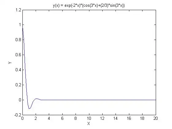
Find and plot the solution for the L2-ODE-CC
Initial conditions: y(0) = 1, y'(0) = 0
No excitation: r(x) = 0

Part 2
In another Fig., superpose 3 Figs.: (a) this Fig.,
(b) the Fig. in R2.6 P. 5-6, (c) the Fig. in R2.1 P. 3-7.
Solution
Part 1

The characteristic equation of the given ODE is:

Using the quadratic formula to solve for

where


Solving to get

,


Therefore, the general solution of the given ODE is
![{\displaystyle y=e^{-2x}[C_{1}\cos 3x+C_{2}\sin 3x]}](../../../../I/df167059eabf2c7acbcc20f8000ec9f449f79177.svg)
Now we solve for , using the given initial conditions


We have

Substituting into ,

We get,
![{\displaystyle 1=e^{-2(0)}[C_{1}\cos 3(0)+C_{2}\sin 3(0)]}](../../../../I/4a62911bdf3a5e5596266d01fd0d72d24e8e7ee6.svg)


We have

Differentiating , we get:
.
![{\displaystyle y'=-2e^{-2x}[C_{1}\cos 3x+C_{2}\sin 3x]+e^{-2x}[-3C_{1}\cos 3x+3C_{2}\sin 3x]}](../../../../I/fd483de9b9595d229b5dcdff19f4c9d53f606b47.svg)
Substituting into , we get:

![{\displaystyle 0=-2e^{-2(0)}[C_{1}\cos 3(0)+C_{2}\sin 3(0)]+e^{-2(0)}[-3C_{1}\cos 3(0)+3C_{2}\sin 3(0)]}](../../../../I/bfc172afd67f776e2820367c313567ec670e81dd.svg)


Therefore, we get

Hence the solution of the given ODE is
![{\displaystyle y=e^{-2x}[\cos 3x+2/3\sin 3x]}](../../../../I/dc28a1b9f6097dfb998f22f25fddf0494cc69dc8.svg)
Fig. 1:
Part 2


Fig. 2:
Fig. 3:
Fig. 4:
Honor Pledge
On our honor, we solved this problem on our own, without aid from online solutions or solutions from previous semesters.
Problem 7
Problem Statement
Consider the same system as in the Example p.7-3, i.e., the same L2-ODE-CC (4) p.5-5 and initial condi- (2) p.3-4, but with the following excitation:

Solution
Replacing with and after simplifying we get,
The root here is . So we can solve for our constants,
Using the initial conditions y(0)=4 and y'(0)=-5 we can solve for our constants,
So the solution is,


Honor Pledge
On our honor, we solved this problem on our own, without aid from online solutions or solutions from previous semesters.
Problem 8
Problem Statement
Plot the error between the exact derivative and the approximate derivative, i.e.
from


For ε = .0001, .0003, .0006, and .001 and λ =.3
Solution
Since the above equation is the error between the exact derivative and the approximate derivative, it must be plotted with the correct values of \epsilon and \lambda, from x = -15 to 15
Case 1
ε=.0001
Case 2
ε=.0003
Case 3
ε=.0006
Case 4
ε=.001

Honor Pledge
On our honor, we solved this problem on our own, without aid from online solutions or solutions from previous semesters.
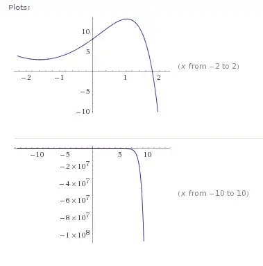
Problem 9
Problem Statement
Find the complete solution for , with the initial conditions
,
plot the solution y(x)

Solution
Particular Solution
Homogeneous Solution
Initial conditions
General Solution


Honor Pledge
On our honor, we solved this problem on our own, without aid from online solutions or solutions from previous semesters.