University of Florida/Egm4313/IEA-f13-team10/R4

Problem Statement

Solve the ODE:

${\displaystyle y''+6y'+9y=8x-2x^{7}}$

With the initial conditions:

${\displaystyle y(0)=1}$

${\displaystyle y'(0)=.5}$

Plot the homogeneous solution

Plot the particular solution

Plot the overall solution

Solution

Homogeneous solution: ${\displaystyle y_{h}(x)=C_{1}e^{-3x}+C_{2}xe^{-3x}}$

So that ${\displaystyle y_{h}'(x)=-3C_{1}e^{-3x}+C_{2}e^{-3x}-3C_{2}xe^{-3x}}$

Solving for the initial conditions:

${\displaystyle y_{h}(0)=1=C_{1}+0}$

${\displaystyle y_{h}'(0)=.5=-3C_{1}+C_{2}-0}$

${\displaystyle C_{1}=1}$
${\displaystyle C_{2}=3.5}$

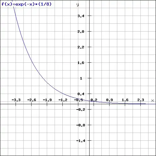
So the homogeneous solution is:

${\displaystyle y_{h}(x)=e^{-3x}+3.5xe^{-3x}}$

Choose the particular solution to be: ${\displaystyle y_{p}(x)=Ax^{7}+Bx^{6}+Cx^{5}+Dx^{4}+Ex^{3}+Fx^{2}+Gx+H}$

So that:

${\displaystyle y_{p}'(x)=7Ax^{6}+6Bx^{5}+5Cx^{4}+4Dx^{3}+3Ex^{2}+2Fx+G}$

${\displaystyle y_{p}''(x)=42Ax^{5}+30Bx^{4}+20Cx^{3}+12Dx^{2}+6Ex+2F}$

Substitute in the original equation ${\displaystyle y''+6y'+9y=8x-2x^{7}}$

${\displaystyle (42Ax^{5}+30Bx^{4}+20Cx^{3}+12Dx^{2}+6Ex+2F)+6(7Ax^{6}+6Bx^{5}+5Cx^{4}+4Dx^{3}+3Ex^{2}+2Fx+G)+...}$
${\displaystyle ...9(Ax^{7}+Bx^{6}+Cx^{5}+Dx^{4}+Ex^{3}+Fx^{2}+Gx+H)=8x-2x^{7}}$

Sorting by the x term gives:

${\displaystyle x^{7}(9A)+x^{6}(42A+9B)+x^{5}(42A+36B+9C)+x^{4}(30B+30C+9D)+...}$
${\displaystyle ...x^{3}(20C+24D+9E)+x^{2}(12D+18E+9F)+x(6E+12F+9G)+(2F+6G+9H)=8x-2x^{7}}$

Giving us the system of equations:


${\displaystyle 9A=-2}$
${\displaystyle 42A+9B=0}$
${\displaystyle 42A+36B+9C=0}$
${\displaystyle 30B+30C+9D=0}$
${\displaystyle 20C+24D+9E=0}$
${\displaystyle 12D+18E+9F=0}$
${\displaystyle 6E+12F+9G=8}$
${\displaystyle 2F+6G+9H=0}$

The Matlab code we made to solve this was:

A = -2/9;

B = -(42*A)/9;

C = -(42*A + 36*B)/9;

D = -(30*B + 30*C)/9;

E = -(20*C + 24*D)/9;

F= -(12*D + 18*E)/9;

G = (8-(6*E + 12*F))/9;

H = -(2*F + 6*G)/9;

To get (rounded to the nearest tenth):

A= -0.2

B= 1.0

C= -3.1

D= 6.9

E= -11.5

F= 13.8

G= -9.9

H= 3.5

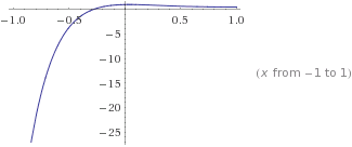
So now the particular solution is:

${\displaystyle y_{p}(x)=-0.2x^{7}+1.0x^{6}-3.1x^{5}+6.9x^{4}-11.5x^{3}+13.8x^{2}-9.9x+3.5}$

The overall solution can be found by:

${\displaystyle y(x)=y_{h}(x)+y_{p}(x)}$

${\displaystyle y(x)=C_{1}e^{-3x}+C_{2}xe^{-3x}-0.2x^{7}+1.0x^{6}-3.1x^{5}+6.9x^{4}-11.5x^{3}+13.8x^{2}-9.9x+3.5}$

To solve for C_1 and C_2 (which are different from the homogeneous solution constants) we find:

${\displaystyle y'(x)=-3C_{1}e^{-3x}+C_{2}e^{-3x}-3C_{2}xe^{-3x}-1.4x^{6}+6.0x^{5}-15.5x^{4}+27.6x^{3}-34.5x^{2}+27.6x-9.9}$

${\displaystyle y(0)=1=C_{1}+3.5}$ ${\displaystyle y'(0)=.5=-3C_{1}+C_{2}-9.9}$

${\displaystyle C_{1}=-2.5}$
${\displaystyle C_{2}=2.8}$

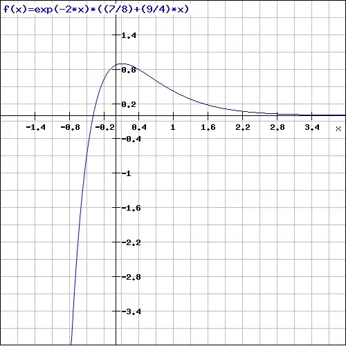
The overall solution is:

${\displaystyle y(x)=-2.5e^{-3x}+2.8xe^{-3x}-0.2x^{7}+1.0x^{6}-3.1x^{5}+6.9x^{4}-11.5x^{3}+13.8x^{2}-9.9x+3.5}$

Plot the homogeneous solution:

Plot the particular solution:

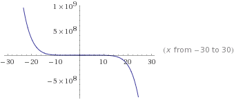
Plot the overall solution:

Honor Pledge

On our honor, we solved this problem on our own, without aid from online solutions or solutions from previous semesters.

Problem Statement

Part 1

Use the Basic Rule 1 and the Sum Rule 3 to show that the appropriate particular solution for:
${\displaystyle y''+6y'+9y=8x-2x^{7}}$
${\displaystyle y(0)=1,\ y'(0)=1/2}$

Part 2

Derive the Basic rule and the Sum rule, instead of just using them, based on the linearity
of the differential operator to obtain the expression (trial solution) for the particular solution ${\displaystyle y_{p}(x)}$

Solution

${\displaystyle y_{p}(x)=\sum _{j=0}^{n}c_{j}x^{j}}$

${\displaystyle y_{p}'(x)=\sum _{j=1}^{n}c_{j}jx^{j-1}=\sum _{j=0}^{n-1}c_{j+1}(j+1)x^{j}}$

${\displaystyle y_{p}''(x)=\sum _{j=2}^{n}c_{j}j(j-1)x^{j-2}=\sum _{j=0}^{n-2}c_{j+2}(j+2)(j+1)x^{j}}$

With n =7 we get

${\displaystyle y_{p}(x)=c_{0}+c_{1}x+c_{2}x^{2}+c_{3}x^{3}+c_{4}x^{4}+c_{5}x^{5}+c_{6}x^{6}+c_{7}x^{7}}$

${\displaystyle y_{p}'(x)=c_{1}+2c_{2}x+3c_{3}x^{2}+4c_{4}x^{3}+5c_{5}x^{4}+6c_{6}x^{5}+7c_{7}x^{6}}$

${\displaystyle y_{p}''(x)=2c_{2}+6c_{3}x+12c_{4}x^{2}+20c_{5}x^{3}+30c_{6}x^{4}+42c_{7}x^{5}}$

From report problem 1 it was already found that:

${\displaystyle c_{0}=3.5}$
${\displaystyle c_{1}=-9.9}$
${\displaystyle c_{2}=13.8}$
${\displaystyle c_{3}=-11.5}$
${\displaystyle c_{4}=6.9}$
${\displaystyle c_{5}=-3.1}$
${\displaystyle c_{6}=1.0}$
${\displaystyle c_{7}=-0.2}$

${\displaystyle y_{p}(x)=-0.2x^{7}+1.0x^{6}-3.1x^{5}+6.9x^{4}-11.5x^{3}+13.8x^{2}-9.9x+3.5}$

Honor Pledge

On our honor, we solved this problem on our own, without aid from online solutions or solutions from previous semesters.

Problem Statement

Problem Set 2.7, problem 5

Find a real, general solution. State which rule you are using. Show each step of your work.

${\displaystyle y''+6y'+9y=e^{x}sin{x}}$
${\displaystyle y(0)=1,\ y'(0)=1/2}$

plot on separate graphs:

(1) the homogeneous solution ${\displaystyle y_{h}(x)}$,

(2) the particular solution ${\displaystyle y_{p}(x)}$,

and (3) the overall solution ${\displaystyle y(x)}$.

Solution

We start by finding the general solution of the homogeneous ODE

${\displaystyle y''+6y'+9y=0}$

The characteristic equation of the homogeneous ODE is

${\displaystyle \lambda ^{2}+6\lambda +9=0}$
${\displaystyle (\lambda +3)^{2}=0}$
${\displaystyle \lambda =-3,-3}$

The roots are double real roots.
The general solution of the homogeneous ODE is ${\displaystyle y_{h}=(c_{1}+xc_{2})e^{-2x}}$

Now we solve for the particular solution of the nonhomogeneous ODE

${\displaystyle y''+6y'+9y=e^{x}sin{x}}$

We use the method of Undetermined Coefficients

${\displaystyle y_{p}=e^{x}(Kcos{x}+Msin{x})}$

${\displaystyle y_{p}'=e^{x}(Kcos{x}+Msin{x})+e^{x}(-Ksin{x}+Mcos{x})}$

${\displaystyle y_{p}''=e^{x}(Kcos{x}+Msin{x})+e^{x}(-Ksin{x}+Mcos{x})+e^{x}(-Ksin{x}+Mcos{x})+e^{x}(-Kcos{x}-Msin{x})}$
${\displaystyle y_{p}''=e^{x}(Kcos{x}+Msin{x})+2e^{x}(-Ksin{x}+Mcos{x})+e^{x}(-Kcos{x}-Msin{x})}$

We now substitute the values of ${\displaystyle y_{p},y_{p}',y_{p}''}$ into ${\displaystyle y''+6y'+9y=e^{x}sin{x}}$

${\displaystyle e^{x}(Kcos{x}+Msin{x})+2e^{x}(-Ksin{x}+Mcos{x})+e^{x}(-Kcos{x}-Msin{x})}$
${\displaystyle +6(e^{x}(Kcos{x}+Msin{x})+e^{x}(-Ksin{x}+Mcos{x}))}$
${\displaystyle +9(e^{x}(Kcos{x}+Msin{x}))=e^{x}sin{x}}$

${\displaystyle 16e^{x}(Kcos{x}+Msin{x})+8e^{x}(-Ksin{x}+Mcos{x})+e^{x}(-Kcos{x}-Msin{x})=e^{x}sin{x}}$
${\displaystyle e^{x}(15(Kcos{x}+Msin{x})+8(-Ksin{x}+Mcos{x})=e^{x}sin{x}}$
${\displaystyle e^{x}((15Kcos{x}+8Mcos{x})+(15Msin{x}-8Ksin{x}))=e^{x}sin{x}}$

Now we equate the coefficients of like terms on both sides
${\displaystyle 15K+8M=0}$
${\displaystyle 15M-8K=1}$

Now we solve these equations for the coefficients
${\displaystyle K=-8/15M}$
${\displaystyle 15M+64/15M=1}$
${\displaystyle M=0.05190}$

${\displaystyle 15K+8(15/289)=0}$
${\displaystyle K=0.02768}$

These values are substituted into ${\displaystyle y_{p}=e^{x}(Kcos{x}+Msin{x})}$ to get the particular solution of the ODE
${\displaystyle y_{p}=e^{x}(0.02768cos{x}+0.05190sin{x})}$

The general solution of the ODE is
${\displaystyle y=y_{h}+y_{p}}$
${\displaystyle y=(c_{1}+xc_{2})e^{-2x}+e^{x}(0.02768cos{x}+0.05190sin{x})}$

In order to determine the values of ${\displaystyle c_{1},c_{2}}$ we use the initial conditions ${\displaystyle y(0)=1,\ y'(0)=1/2}$
${\displaystyle y(0)=c_{1}+0.02768=1}$
${\displaystyle c_{1}=0.97232}$

${\displaystyle y'=-2e^{-2x}(c_{1}+xc_{2})+e^{-2x}(c_{2})+e^{x}(0.02768cos{x}+0.05190sin{x})+e^{x}(-0.02768sin{x}+0.05190cos{x})}$
${\displaystyle y'=-2e^{-2x}(c_{1}+xc_{2})+e^{-2x}(c_{2})+e^{x}(0.07958cos{x}+0.02422sin{x})}$
${\displaystyle y(0)'=-2(c_{1})+c_{2}+0.07958=1/2}$
${\displaystyle y(0)'=-1.94464+c_{2}+0.07958=1/2}$
${\displaystyle c_{2}=2.36506}$

The general solution of the ODE is
${\displaystyle y=e^{-2x}(0.97232+2.36506x)+e^{x}(0.02768cos{x}+0.05190sin{x})}$

Plot the homogeneous solution:

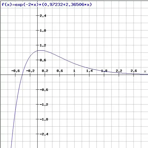
Plot the particular solution:

Plot the overall solution:

Honor Pledge

On our honor, we solved this problem on our own, without aid from online solutions or solutions from previous semesters.

Problem Statement

Problem Set 2.7, problem 5

Find a real, general solution. State which rule you are using. Show each step of your work.

${\displaystyle y''+6y'+9y=e^{-2x}\sinh x}$
${\displaystyle y(0)=1,\ y'(0)=1/2}$

plot on separate graphs:

(1) the homogeneous solution ${\displaystyle y_{h}(x)}$,

(2) the particular solution ${\displaystyle y_{p}(x)}$,

and (3) the overall solution ${\displaystyle y(x)}$.

Solution

We start by finding the general solution of the homogeneous ODE

${\displaystyle y''+6y'+9y=0}$

The characteristic equation of the homogeneous ODE is

${\displaystyle \lambda ^{2}+6\lambda +9=0}$
${\displaystyle (\lambda +3)^{2}=0}$
${\displaystyle \lambda =-3,-3}$

The roots are double real roots.
The general solution of the homogeneous ODE is ${\displaystyle y_{h}=e^{-2x}(c_{1}+xc_{2})}$

Now we solve for the particular solution of the non-homogeneous ODE

${\displaystyle y''+6y'+9y=e^{-2x}\sinh x}$

By using the definition of hyperbolic trigonometric functions we can convert ${\displaystyle \sinh x=1/2(e^{x}-e^{-x})}$.
Our non-homogeneous ODE can now be written as:

${\displaystyle y''+6y'+9y=e^{-2x}(1/2(e^{x}-e^{-x})}$

${\displaystyle y''+6y'+9y=1/2(e^{-x}-e^{-3x})}$

Since the replacement of ${\displaystyle \sinh x}$ is the sum of two functions we can use the sum rule for the method of undetermined coefficients.

${\displaystyle y_{p}=y_{p1}+y_{p2}=Je^{-x}-Ke^{-3x}}$

${\displaystyle y_{p}=Je^{-x}-Ke^{-3x}}$

${\displaystyle y'_{p}=-Je^{-x}+3Ke^{-3x}}$

${\displaystyle y''_{p}=Je^{-x}-9Ke^{-3x}}$

We now substitute the values of ${\displaystyle y_{p},y_{p}',y_{p}''}$ into ${\displaystyle y''+6y'+9y=1/2(e^{-x}-e^{-3x})}$

${\displaystyle Je^{-x}-9Ke^{-3x}}$
${\displaystyle +6(-Je^{-x}+3Ke^{-3x})}$
${\displaystyle +9(Je^{-x}-Ke^{-3x})=1/2(e^{-x}-e^{-3x})}$

${\displaystyle Je^{-x}-9Ke^{-3x}-6Je^{-x}+18Ke^{-3x}+9Je^{-x}-9Ke^{-3x}=1/2(e^{-x}-e^{-3x})}$

${\displaystyle 4Je^{-x}=1/2(e^{-x}-e^{-3x})}$

Now we equate the coefficients of like terms on both sides and solve for the coefficients
${\displaystyle 4J=1/2}$
${\displaystyle J=1/8}$
${\displaystyle K=0}$

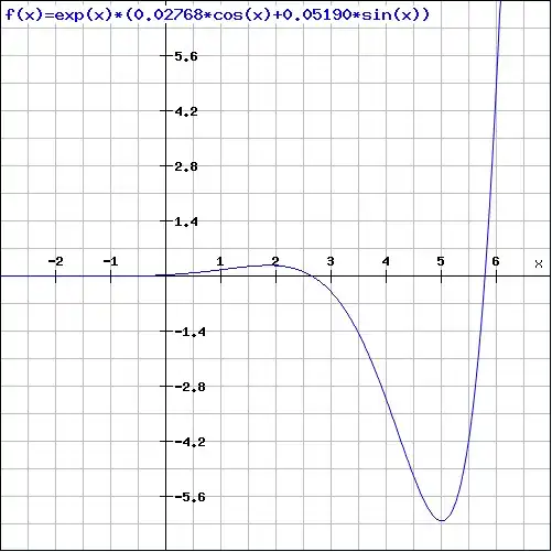
These values are substituted into ${\displaystyle y_{p}=Je^{-x}-Ke^{-3x}}$ to get the particular solution of the ODE

${\displaystyle y_{p}=1/8e^{-x}}$

The general solution of the ODE is:

${\displaystyle y=y_{h}+y_{p}}$
${\displaystyle y=e^{-2x}(c_{1}+xc_{2})+1/8e^{-x}}$

In order to determine the values of ${\displaystyle c_{1},c_{2}}$ we use the initial conditions ${\displaystyle y(0)=1,\ y'(0)=1/2}$
${\displaystyle y(0)=c_{1}+1/8=1}$
${\displaystyle c_{1}=7/8}$

${\displaystyle y'=-2e^{-2x}(c_{1}+xc_{2})+e^{-2x}c_{2}}$
${\displaystyle y'=-2e^{-2x}(7/8+xc_{2})+e^{-2x}c_{2}}$
${\displaystyle y(0)'=-14/8+c_{2}=1/2}$
${\displaystyle c_{2}=9/4}$

The general solution of the ODE is
${\displaystyle y=e^{-2x}(7/8+9/4x)+1/8e^{-x}}$

Plot the homogeneous solution:

Plot the particular solution:

Plot the general solution:

Honor Pledge

On our honor, we solved this problem on our own, without aid from online solutions or solutions from previous semesters.

Problem Statement

Expand the series on both sides of (1)-(2) p.7-12b to verify these equalities
${\displaystyle (1)}$

${\displaystyle \sum _{j=2}^{5}c_{j}*j*(j-1)*x^{j-2}=\sum _{j=0}^{3}c_{j+2}*(j+2)*(j+1)*x^{j}}$

${\displaystyle (2)}$

${\displaystyle \sum _{j=1}^{5}c_{j}*j*x^{j-1}=\sum _{j=0}^{4}c_{j+1}*(j+1)*x^{j}}$

Solution

Evaluating the right-hand side of (1):

${\displaystyle c_{2}2(2-1)x^{2-2}+c_{3}3(3-1)x^{3-2}+c_{4}4(4-1)x^{4-2}+c_{5}5(5-1)x^{5-2}}$

${\displaystyle =2c_{2}+6c_{3}x+12c_{4}x^{2}+20c_{5}x^{3}}$

Now evaluating the left-hand side of (1):

${\displaystyle c_{0+2}(0+2)(0+1)x^{0}+c_{1+2}(1+2)(1+1)x^{1}+c_{2+2}(2+2)(2+1)x^{2}+c_{3+2}(3+2)(3+1)x^{3}}$

${\displaystyle =2c_{2}+6c_{3}x+12c_{4}x^{2}+20c_{5}x^{3}}$

So both sides are equal.

Now evaluating the right-hand side of (2):

${\displaystyle c_{1}(1)x^{1-1}+c_{2}(2)x^{2-1}+c_{3}(3)x^{3-1}+c_{4}(4)x^{4-1}+c_{5}(5)x^{5-1}}$

${\displaystyle =c_{1}+2c_{2}x+3c_{3}x^{2}+4c_{4}x^{3}+5c_{5}x^{4}}$

The left-hand side of (2) expands into the following:

${\displaystyle c_{0+1}(0+1)x^{0}+c_{1+1}(1+1)x^{1}+c_{1+1}(1+1)x^{1}+c_{2+1}(2+1)x^{2}+c_{3+1}(3+1)x^{3}+c_{4+1}(4+1)x^{4}}$

${\displaystyle =c_{1}+2c_{2}x+3c_{3}x^{2}+4c_{4}x^{3}+5c_{5}x^{4}}$

So both sides are equal.

Honor Pledge

On our honor, we solved this problem on our own, without aid from online solutions or solutions from previous semesters.

Problem Statement

${\displaystyle y''+6y'+9y=cos(2x)}$
${\displaystyle y(0)=1}$ and ${\displaystyle y'(0)=1/2}$

Solution

The taylor series for the excitation is ${\displaystyle \sum {\frac {(-4)^{n}*x^{2n}}{(2n)!}}}$ from n=0 to infinity
For n=3, this equals ${\displaystyle 1-2x^{2}+2x^{4}/3-4x^{6}/45}$
For n=5, this equals ${\displaystyle 1-2x^{2}+2x^{4}/3-4x^{6}/45+2x^{8}/315-4x^{10}/14175}$
For n=9, this equals ${\displaystyle 1-2x^{2}+2x^{4}/3-4x^{6}/45+2x^{8}/315-4x^{10}/14175+4x^{12}/467775-8x^{14}/42567525+2x^{16}/638512875-4x^{18}/97692469875}$

For n=3,
${\displaystyle y_{p}=Ax^{6}+Bx^{5}+Cx^{4}+Dx^{3}+Ex^{2}+Fx+G}$
${\displaystyle y'_{p}=6Ax^{5}+5Bx^{4}+4Cx^{3}+3Dx^{2}+2Ex+F}$
${\displaystyle y''_{p}=30Ax^{4}+20Bx^{3}+12Cx^{2}+6Dx+2E}$

Plugging these into the original equation using the taylor series approximation as the excitation,
${\displaystyle (Ax^{6}+Bx^{5}+Cx^{4}+Dx^{3}+Ex^{2}+Fx+G)+6(6Ax^{5}+5Bx^{4}+4Cx^{3}+3Dx^{2}+2Ex+F)+9(30Ax^{4}+20Bx^{3}+12Cx^{2}+6Dx+2E)}$
${\displaystyle =1-2x^{2}+2x^{4}/3-4x^{6}/45}$
Rearranging the coefficients,
${\displaystyle Ax^{6}+(B+36A)x^{5}+(C+30B+270A)x^{4}+(D+24C+180B)x^{3}+(E+18D+108C)x^{2}+(F+12E+54D)x+(G+6F+18E)}$
${\displaystyle =1+0x-2x^{2}+0x^{3}+2x^{4}/3+0x^{5}-4x^{6}/45}$


Equating x^6 coefficients, A=-45/4
Equating x^5 coefficients, B=405
Equating x^4 coefficients, C=-118461.833
Equating x^3 coefficients, D=2770183.992
Equating x^2 coefficients, E=-37069430.492
Equating x^1 coefficients, F=-594423101.472
Equating x^0 coefficients, G=4233788358.69
${\displaystyle y_{p}=-45/4x^{6}+405x^{5}+-118461.833x^{4}+2770183.992x^{3}-37069430.492x^{2}-594423101x+4233788358.69}$

The graph shown is the taylor series for cos(2x) for the 0th through 3rd order.

Honor Pledge

On our honor, we solved this problem on our own, without aid from online solutions or solutions from previous semesters.

Problem Statement

${\displaystyle y''+6y'+9y=log(3+4x)}$
${\displaystyle y(0)=1,y'(0)=.5}$
Use the point
${\displaystyle {\widehat {x}}=-1/2}$
${\displaystyle \log x=\log _{e}x=\ln x}$

Solution

The taylor series expansion for ${\displaystyle log(3+4x)}$ around ${\displaystyle {\widehat {x}}=-1/2}$ up to 16 terms is
${\displaystyle 4(x+.5)-8(x+.5)^{2}+{\frac {64}{3}}(x+.5)^{3}-{64}(x+.5)^{4}+{\frac {1024}{5}}(x+.5)^{5}-{\frac {2048}{3}}(x+.5)^{6}+{\frac {16384}{7}}(x+.5)^{7}-8192(x+.5)^{8}}$
${\displaystyle +{\frac {262144}{9}}(x+.5)^{9}-{\frac {524288}{5}}(x+.5)^{10}+{\frac {4194304}{11}}(x+.5)^{11}-{\frac {4194304}{3}}(x+.5)^{12}+{\frac {67108864}{13}}(x+.5)^{13}}$
${\displaystyle -{\frac {134217728}{7}}(x+.5)^{14}+{\frac {1073741824}{15}}(x+.5)^{15}-{\frac {268435456}{3}}(x+.5)^{16}}$
Plots of taylor series expansion: Up to order 4


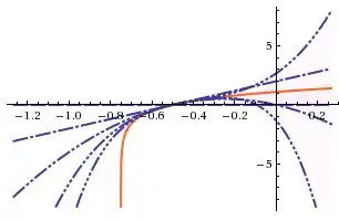
Up to order 7


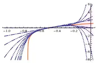
Up to order 11


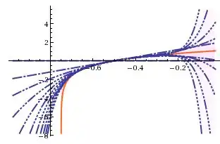
Up to order 16


The visually estimated domain of convergence is from .8 to .2.
Now use the transformation of variable
${\displaystyle x\longrightarrow t\ {\text{ such that }}\ 3+4x=1+t}$
${\displaystyle x={\frac {t-2}{4}}}$

If ${\displaystyle log(1+t)}$ has a domain of convergence from ${\displaystyle [-1,+1]}$ then ${\displaystyle log(3+4x)}$ converges from ${\displaystyle [{\frac {-3}{4}},{\frac {-1}{4}}]}$

Honor Pledge

On our honor, we solved this problem on our own, without aid from online solutions or solutions from previous semesters.