University of Florida/Egm4313/s12.team11.R5
Report 5
Intermediate Engineering Analysis
Section 7566
Team 11
Due date: March 30, 2012.
R5.1
Problem Statement
Given: Find for the following series:
1.
2.
Find for the Taylor series of
3. at


4. at

5. at

Solution
The radius of convergence is defined as
1.
![{\displaystyle R_{c}=[\lim _{k\to \infty }|{\frac {d_{k+1}}{d_{k}}}|]^{-1}\!}](../../../I/d6b8ccc715a7471923f69e28178706700849ca1f.svg)
![{\displaystyle R_{c}=[\lim _{k\to \infty }|{\frac {(k+2)(k+1)}{(k+1)(k)}}|]^{-1}\!}](../../../I/fc71081c7afee94390e37f71f56d2193dec48de9.svg)
![{\displaystyle R_{c}=[\lim _{k\to \infty }|{\frac {(k+2)}{(k)}}|]^{-1}\!}](../../../I/b1af688ca1f47d693121b1271218fd929490e415.svg)
![{\displaystyle R_{c}=[\lim _{k\to \infty }|{\frac {k(1+{\frac {2}{k}})}{k}}|]^{-1}\!}](../../../I/91507d0db845548c113c47343de793dc125cf834.svg)
![{\displaystyle R_{c}=[\lim _{k\to \infty }|1+{\frac {2}{k}}|]^{-1}\!}](../../../I/5c8a3989bc7fc0b444be04b556b2d2ee1c1a1d7d.svg)
![{\displaystyle R_{c}=[1+0]^{-1}\!}](../../../I/ea6fe870b92b59fdd2dd61e493f66c583d007ff5.svg)

2.
![{\displaystyle R_{c}=[\lim _{k\to \infty }|{\frac {\frac {(-1)^{k+1}}{\gamma ^{k+1}}}{\frac {(-1)^{k}}{\gamma ^{k}}}}|]^{-1}\!}](../../../I/05386557debdb49583acce7ab9f83a1d4be70b88.svg)
![{\displaystyle R_{c}=[\lim _{k\to \infty }|{\frac {-1}{\gamma }}|]^{-1}\!}](../../../I/f4544068f0608761e16857dd77cca7662123056f.svg)
![{\displaystyle R_{c}=[\lim _{k\to \infty }{\frac {1}{\gamma }}]^{-1}\!}](../../../I/7997241d23909c23c91497322fbe1ff149d57d78.svg)
![{\displaystyle R_{c}=[{\frac {1}{\gamma }}]^{-1}\!}](../../../I/1414ef0ffee2c582ed3eeaf9a7993a628b08b4d0.svg)

However, in this problem, the series term is not , as is the general form.
Therefore, this implies:


3. The Taylor series for is expressed as
Therefore:


![{\displaystyle R_{c}=[\lim _{k\to \infty }{\frac {1}{(2k+3)}}]^{-1}\!}](../../../I/3b3f749928e2e6110c615a89db49b3e83b1ca1c5.svg)

4. The Taylor series for at is expressed as

![{\displaystyle R_{c}=[\lim _{k\to \infty }|{\frac {\frac {(-1)^{k+2}}{k+1}}{\frac {(-1)^{k+1}}{k}}}|]^{-1}\!}](../../../I/1c89f760e5fa1462fac57cfd53e47c7ba4695f4d.svg)
![{\displaystyle R_{c}=[\lim _{k\to \infty }|{\frac {\frac {(-1)}{k+1}}{\frac {(1)}{k}}}|]^{-1}\!}](../../../I/e0fd04d810dc90cb7de776420e8b664f3ff32f6f.svg)
![{\displaystyle R_{c}=[\lim _{k\to \infty }|{\frac {\frac {(-1)}{k(1+{\frac {1}{k}})}}{\frac {1}{k}}}|]^{-1}\!}](../../../I/27d01121f5bf24b5b3c0f00bdc9fe4cea9fabdaf.svg)
![{\displaystyle R_{c}=[\lim _{k\to \infty }|{\frac {(-1)}{(1+{\frac {1}{k}})}}|]^{-1}\!}](../../../I/de135421582f0cd5c0506882a31fb79c9d191882.svg)
![{\displaystyle R_{c}=[1/1]^{-1}\!}](../../../I/18d3becf975c7c5cb357e14fbb8da3130baba3f1.svg)
5. The Taylor series for at is expressed as
For convergence:
Therefore,


R5.2
Solved by: Andrea Vargas
Problem Statement
Part 1:Determine whether the following are linearly independent using the Wronskian
Part 2: Determine whether the following are linearly independent using the Gramian
Solution
Part 1
Using the Wronskian we check for linear independence.
We know from (1) and (2) in 7-35 that if
Then the functions are linearly independent.

Part 1.1


Taking the derivatives of each function:


f(x) and g(x) are linearly independent

Part 1.2


Taking the derivatives of each function:


f(x) and g(x) are linearly independent
Part 2
Using the Gramian we check for linear independence.
We know from the notes in (1) 7-34 that:

and that the Gramian is defined as:

Then f,g are linearly independent if

Part 2.1
Taking scalar products:
![{\displaystyle \langle f,f\rangle :=\int _{-1}^{1}=f(x)f(x)=x^{2}*x^{2}=\int _{-1}^{1}=x^{4}=\left[{\frac {x^{5}}{5}}\right]_{-1}^{1}={\frac {2}{5}}\!}](../../../I/c9558e9969a77a0045d0716d1f5ae91e7ddad89e.svg)
![{\displaystyle \langle f,g\rangle =\langle g,f\rangle :=\int _{-1}^{1}=f(x)g(x)=x^{2}*x^{4}=\int _{-1}^{1}=x^{6}=\left[{\frac {x^{7}}{7}}\right]_{-1}^{1}={\frac {2}{7}}\!}](../../../I/602b892d340a3d3b15cdad195048562b0b4c3d81.svg)
![{\displaystyle \langle g,g\rangle :=\int _{-1}^{1}=g(x)g(x)=x^{4}*x^{4}=\int _{-1}^{1}=x^{8}=\left[{\frac {x^{9}}{9}}\right]_{-1}^{1}={\frac {2}{9}}\!}](../../../I/c7ea937455865cedfe397a7909635c90e2c5c920.svg)

f(x) and g(x) are linearly independent
Part 2.2
Taking scalar products:
We can use the trig identity for power reduction
Then we have,


![{\displaystyle \int _{-1}^{1}{\frac {1}{2}}\cos(2x)+{\frac {1}{2}}dx=\left[{\frac {1}{4}}\sin(2x)+{\frac {1}{2}}x\right]_{-1}^{1}\!}](../../../I/1b430bf3d0b57d4d80031e1c87c89e7e84cf1a67.svg)


![{\displaystyle =\int _{-1}^{1}\sin(3x)\cos(x)dx=\left[{\frac {1}{8}}(-2\cos(2x)-\cos(4x))\right]_{-1}^{1}\!}](../../../I/8203ee3878256536c05c42f6634ab0d963539e6e.svg)


![{\displaystyle ={\frac {1}{2}}\int _{-1}^{1}1-\cos(6x)dx=\left[{\frac {1}{2}}(x-{\frac {1}{6}}\sin(6x))\right]_{-1}^{1}\!}](../../../I/2ce4d0a3d02f4039abbee99ac372ff1fb6572374.svg)


f(x) and g(x) are linearly independent
Conclusion
By both methods (the Wronskian and the Gramian) we obtain the same results.
R5.3
Problem Statement
Verify using the Gramian that the following two vectors are linearly independent.


Solution

We know from (3) 8-9 that:

We obtain,


Then,

b_1 and b_2 are linearly independent
R5.4
Problem Statement
Show that is indeed the overall particular solution of the L2-ODE-VC with the excitation .


Discuss the choice of in the above table e.g., for why would you need to have both and in ?


Solution
Because the ODE is a linear equation in y and its derivatives with respect to x, the superposition principle can be applied:
is a specific excitation with known form of and is a specific excitation with known form of


becomes

proving that
is indeed the overall particular solution of the L2-ODE-VC with the excitation

According to Fourier Theorem periodic functions can be represented as infinite series in terms of cosines and sines:
![{\displaystyle f(x)=a_{0}+\sum _{n=1}^{\infty }[a_{n}\cos \omega x+b_{n}\sin \omega x]\!}](../../../I/1abd51ec088c597412c9e0bbb11e2628601e639e.svg)
where the coefficients are the Fourier coefficients calculated using Euler formulas.

So even though the system is being excited by functions like the particular solution would still include both and in because the excitation is a periodic function that can be represented as the Fourier infinite series in terms of both and times the Fourier coefficients
R5.5
Part 1
Problem Statement
Show that and are linearly independant using the Wronskian and the Gramain (integrate over 1 period)


Solution
One period of
Wronskian of f and g


Plugging in values for


![{\displaystyle =7[cos^{2}(7x)+sin^{2}(7x)]}](../../../I/b301de567d6ca791f8580ee8e9e260a31d103757.svg)
![{\displaystyle =7[1]}](../../../I/b92b8a5eea92d540f3a060ab9d154589aa005e48.svg)
They are linearly Independant using the Wronskian.


They are linearly Independent using the Gramain.
Problem Statement
Find 2 equations for the 2 unknowns M,N and solve for M,N.
Solution
Plugging these values into the equation given () yields;
Simplifying and the equating the coefficients relating sin and cos results in;
Solving for M and N results in;


Problem Statement
Find the overall solution that corresponds to the initial conditions . Plot over three periods.


Solution
From before, one period so therefore, three periods is
Using the roots given in the notes , the homogenous solution becomes;
Using initial condtion ;
with
Solving for the constants;
Using the found in the last part;


R5.6
solved by Luca Imponenti
Problem Statement
Complete the solution to the following problem

where
![{\displaystyle y_{h}=e^{-2x}[Acos(3x)+Bsin(3x)]\!}](../../../I/792e67f127ff688d55ed48d9f0303345b9a28184.svg)
and
![{\displaystyle y_{p}=xe^{-2x}[Mcos(3x)+Nsin(3x)]\!}](../../../I/96a697d5683642f371e1127b4a15314d1a2b93f0.svg)
Find the overall solution corresponds to the initial condition:


Plot the solution over 3 periods.
Particular Solution
Taking the derivatives of the particular solution
![{\displaystyle y'_{p}=e^{-2x}[sin(3x)(N-2Nx-3Mx)+cos(3x)(3Nx+M-2Mx)]\!}](../../../I/4229480759610de8da772b0745c06b16b70b56ae.svg)
![{\displaystyle y''_{p}=e^{-2x}[sin(3x)(12Mx-6M-5Nx-4N)+cos(3x)(6N-5Mx-4M-12Nx)]\!}](../../../I/57b163ea521277f918af0d523c1e8f0ca8e234ff.svg)
Plugging these into the ODE yields

![{\displaystyle 4[sin(3x)(N-2Nx-3Mx)+cos(3x)(3Nx+M-2Mx)]+}](../../../I/2edffedd7a2b90e82102acd19a704b0b273dc2fd.svg)
![{\displaystyle 13x[Mcos(3x)+Nsin(3x)]=2cos(3x)\!}](../../../I/d9655d1493f66fa3a0f7589a9c3631d9b4476def.svg)
Equating like terms allows us to solve for M and N
![{\displaystyle sin(3x)[(12Mx-6M-5Nx-4N)+4(N-2Nx-3Mx)+13Nx]=0\!}](../../../I/a020f3dd194ee3d5cfeabb37b2da5e9f270c8290.svg)
![{\displaystyle cos(3x)[(6N-5Mx-4M-12Nx)+4(3Nx+M-2Mx)+13Mx]=2cos(3x)\!}](../../../I/61f7febe8c0331fa45a5d99aafb6b7551136061a.svg)


So the particular solution is

Overall Solution
The overall solution in the sum of the homogeneous and particular solutions

![{\displaystyle y(x)=e^{-2x}[Acos(3x)+Bsin(3x)]+{\frac {1}{3}}xe^{-2x}sin(3x)\!}](../../../I/b9ba4455133d526b6750b7d4ad088a2b3ebeb60a.svg)
To find A and B we apply the initial conditions

Taking the derivative
![{\displaystyle y'(x)={\frac {d}{dx}}[e^{-2x}[cos(3x)+Bsin(3x)]+{\frac {1}{3}}xe^{-2x}sin(3x)]\!}](../../../I/8363fdca8c2a01fd5519870363c110a30f746261.svg)
![{\displaystyle y'(x)=e^{-2x}[(3B+x-2)cos(3x)-(2B+{\frac {2}{3}}x+{\frac {8}{3}})sin(3x)]\!}](../../../I/c86f7dc58a6220ae49af31a9fe4e261acfa83019.svg)


Giving us the overall solution
![{\displaystyle y(x)=e^{-2x}[cos(3x)+{\frac {2}{3}}sin(3x)+{\frac {1}{3}}xsin(3x)]\!}](../../../I/c0df58d196d9072113ac3bbd23846cbeaa804059.svg)
Plot
The period for is


Plotting the solution over 3 periods yields

R5.7
Solved by Daniel Suh
Problem Statement


1. Find the components using the Gram matrix.
2. Verify the result by using and , and rely on the non-zero determinant matrix of and relative to the bases of and .


Part 1 Solution
Gram Matrix
Thus,


![{\displaystyle \Gamma =det[T]=(53)(11.25)-(24)(24)=20.25\!}](../../../I/7a18e1ee1c3750d81d34b124c3b39230952ce917.svg)
Defining c
Define:


If , then exists


Finding c
thus, exists


Part 2 Solution


solution is correct
R5.8
Problem Statement
Find the integral
for and
Using integration by parts, and then with the help of of
General Binomial Theorem


Solution
For :
For substitution by parts,
Therefore:


Using the General Binomial Theorem:
Therefore:
Which we have previously found that answer as:


For :
Initially we use the following substitutions:
First let us consider the first term:
Next, we use the integration by parts:
Next let us consider the second term:
Again, we will use integration by parts:
Therefore:
Re-substituting for t:
Therefore:


Using the General Binomial Theorem for the integral with t substitution :
Therefore:
Which we have previously found that answer as:


R5.9
Solved by: Gonzalo Perez
Problem Statement
Consider the L2-ODE-CC (5) p.7b-7 with as excitation:
(5) p.7b-7

(1) p.7c-28

and the initial conditions
.

Part 1
Part A
Project the excitation on the polynomial basis

(1)

i.e., find such that

(2)

for x in , and for n = 3, 6, 9.
![{\displaystyle [{\frac {-3}{4}},3]\!}](../../../I/efbbc5a8b7f6494e546480187267b0e87c07e6fd.svg)
Plot and to show uniform approximation and convergence.

Note that:
(3)

Solution
To solve this problem, it is important to know that the scalar product is defined as the following:
.

Therefore, it follows that:
, where and .


We know that if are linearly independent, then by theorem on p.7c-37, the matrix is solvable.

According to this and (3)p.8-14:
If exists . (3)p.8-14


Now let's define the Gram matrix as a function of :


(1)p.8-13

Defining the "d" matrix as was done in (3)p.8-13, we get:
. (3)p.8-13

And according to (1)p.8-15: (1)p.8-15

Now, we can find the values to compare to .


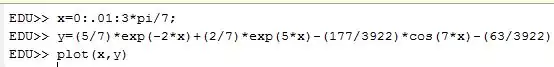
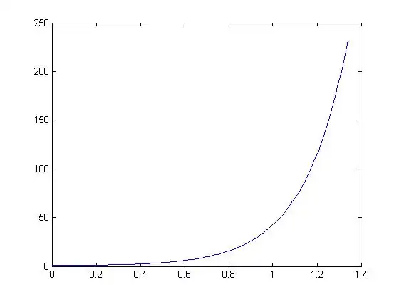
Using Matlab, this is the code that was used to produce the results:
The Matlab code above produced the following graph:
Where is represented by the dashed line and the approximation,, is represented by the red line. This code can work for all n values.
Part B
In a seperate series of plots, compare the approximation of the function by Taylor series expansion about .

Where:

Solution
For n=1:

For n=2:

For n=3:

For n=4:

For n=5:

For n=6:

For n=7:

For n=8:

For n=9:

For n=10:

For n=11:

For n=12:

For n=13:

For n=14:

For n=15:

For n=16:

Using Matlab to plot the graph:
Part 2
Find such that:

(1) p.7c-27

with the same initial conditions as in (2) p.7c-28.
Plot for n = 3, 6, 9, for x in .
In a series of separate plots, compare the results obtained with the projected excitation on polynomial basis to those with truncated Taylor series of the excitation. Plot also the numerical solution as a baseline for comparison.
Solution
First, we find the homogeneous solution to the ODE:
The characteristic equation is:
Then,
Therefore the homogeneous solution is:


Now to find the particulate solution
For n=3:


We can then use a matrix to organize the known coefficients:
Then, using MATLAB and the backlash operator we can solve for these unknowns:
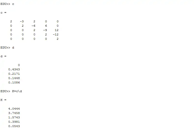
Therefore
Superposing the homogeneous and particulate solution we get
Differentiating:
Evaluating at the initial conditions:
We obtain:
Finally we have:


For n=6:

We can then use a matrix to organize the known coefficients:
Then, using MATLAB and the backlash operator we can solve for these unknowns:
Therefore
Superposing the homogeneous and particulate solution we get
Differentiating:
Evaluating at the initial conditions:
We obtain:
Finally


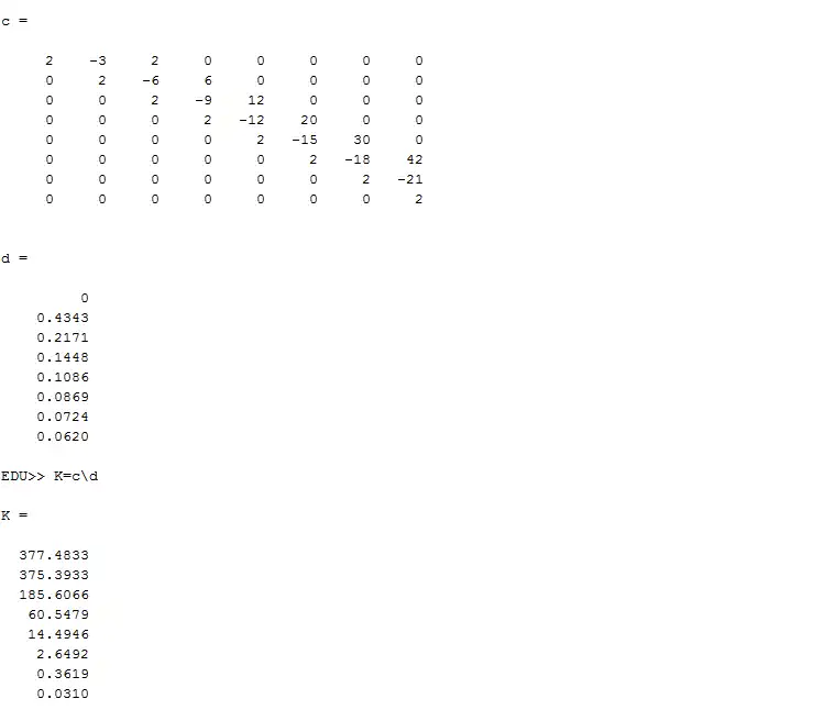
For n=9:

We can then use a matrix to organize the known coefficients:
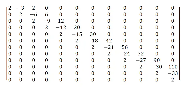
Then, using MATLAB and the backlash operator we can solve for these unknowns:

Therefore
Superposing the homogeneous and particulate solution we get
Differentiating:
Evaluating at the initial conditions:
We obtain:
Finally


Here is the graph for this problem using Matlab: