University of Florida/Egm4313/s12.team11.imponenti/R4.4

Homogeneous Solution

The homogeneous case is shown below:

${\displaystyle y''_{h}-3y'_{h}+2y_{h}=0\!}$

This equation has the following roots:

${\displaystyle \lambda _{1}=1,\lambda _{2}=2\!}$

Which gives yields the homogeneous solution

${\displaystyle y_{h}=c_{1}e^{x}+c_{2}e^{2x}\!}$

General Solution, n=4

Using the taylor series approximation from earlier with ${\displaystyle n=4\!}$ we have

${\displaystyle r_{4}(x)=log(2)+{\frac {(x-1)}{2ln(10)}}-{\frac {(x-1)^{2}}{8ln(10)}}+{\frac {(x-1)^{3}}{24ln(10)}}-{\frac {(x-1)^{4}}{64ln(10)}}\!}$

We know the particular solution, ${\displaystyle y_{p4}(x)\!}$, ve will have this form:

${\displaystyle y_{p4}(x)=a_{4}(x-1)^{4}+a_{3}(x-1)^{3}+a_{2}(x-1)^{2}+a_{1}(x-1)+a_{0}\!}$

taking the derivatives of this solution

${\displaystyle y'_{p4}(x)={\frac {d}{dx}}y_{p4}(x)=4a_{4}(x-1)^{3}+3a_{3}(x-1)^{2}+2a_{2}(x-1)+a_{1}\!}$

and

${\displaystyle y''_{p4}(x)={\frac {d}{dx}}y'_{p4}(x)=12a_{4}(x-1)^{3}+6a_{3}(x-1)^{2}+2a_{2}\!}$

Plugging the above equations into the original ODE yields the following matrix equation:

${\displaystyle {\begin{bmatrix}2&0&0&0&0\\-12&2&0&0&0\\12&-9&2&0&0\\0&6&-6&2&0\\0&0&2&-3&2\end{bmatrix}}*{\begin{bmatrix}a_{4}\\a_{3}\\a_{2}\\a_{1}\\a_{0}\end{bmatrix}}={\begin{bmatrix}-{\frac {1}{64ln(10)}}\\{\frac {1}{24ln(10)}}\\-{\frac {1}{8ln(10)}}\\{\frac {1}{2ln(10)}}\\log(2)\end{bmatrix}}\!}$

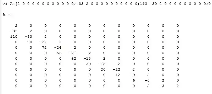
The unknown vector ${\displaystyle a\!}$ can be easily solved by forward substitution,the following values were calculated in matlab:

${\displaystyle a_{4}=-.0034,a_{3}=-.0113,a_{2}=-.0577,a_{1}=-.1624,a_{0}=.1624\!}$

So the particular solution ${\displaystyle y_{p4}\!}$ is

${\displaystyle y_{p4}=0.1624-0.1624*(x-1)-.0577*(x-1)^{2}-.0113*(x-1)^{3}-.0034*(x-1)^{4}\!}$

We can now find the general solution for n=4, ${\displaystyle y_{4}(x)\!}$.

${\displaystyle y_{4}(x)=y_{h}(x)+y_{p4}(x)\!}$

${\displaystyle y_{4}(x)=c_{1}e^{x}+c_{2}e^{2x}+0.1624-0.1624*(x-1)\!}$ ${\displaystyle -.0577*(x-1)^{2}-.0113*(x-1)^{3}-.0034*(x-1)^{4}\!}$

Solving using the initial conditions yields;

        ${\displaystyle y_{4}(x)=.0595e^{x}-.0076e^{2x}+0.1624-0.1624*(x-1)\!}$
          ${\displaystyle -.0577*(x-1)^{2}-.0113*(x-1)^{3}-.0034*(x-1)^{4}\!}$

General Solution, n=7

Using the taylor series approximation from earlier with ${\displaystyle n=7\!}$ we have

${\displaystyle r_{7}(x)=log(2)+{\frac {(x-1)}{2ln(10)}}-{\frac {(x-1)^{2}}{8ln(10)}}+{\frac {(x-1)^{3}}{24ln(10)}}-{\frac {(x-1)^{4}}{64ln(10)}}+{\frac {(x-1)^{5}}{160ln(10)}}-{\frac {(x-1)^{6}}{384ln(10)}}+{\frac {(x-1)^{7}}{896ln(10)}}\!}$

In a similar fashion we construct a matrix equation for n=7:

${\displaystyle {\begin{bmatrix}2&0&0&0&0&0&0&0\\-21&2&0&0&0&0&0&0\\42&-18&2&0&0&0&0&0\\0&30&-15&2&0&0&0&0\\0&0&20&-12&2&0&0&0\\0&0&0&12&-9&2&0&0\\0&0&0&0&6&-6&2&0\\0&0&0&0&0&2&-3&2\end{bmatrix}}*{\begin{bmatrix}a_{7}\\a_{6}\\a_{5}\\a_{4}\\a_{3}\\a_{2}\\a_{1}\\a_{0}\end{bmatrix}}={\begin{bmatrix}{\frac {1}{896ln(10)}}\\-{\frac {1}{384ln(10)}}\\{\frac {1}{160ln(10)}}\\-{\frac {1}{64ln(10)}}\\{\frac {1}{24ln(10)}}\\-{\frac {1}{8ln(10)}}\\{\frac {1}{2ln(10)}}\\log(2)\end{bmatrix}}\!}$

Solving:

${\displaystyle a_{7}=.0002,a_{6}=.0020,a_{5}=.0141,a_{4}=.0725,a_{3}=.3034,a_{2}=.9029,a_{1}=1.9072,a_{0}=2.1084\!}$

So the particular solution ${\displaystyle y_{p7}\!}$ is

${\displaystyle y_{p7}=2.1084+1.9072*(x-1)+.9029*(x-1)^{2}+.3034*(x-1)^{3}+.0725*(x-1)^{4}+.0141*(x-1)^{5}+.0020*(x-1)^{6}+.0002*(x-1)^{7}\!}$

We can now find the general solution for n=7, ${\displaystyle y_{7}(x)\!}$.

${\displaystyle y_{7}(x)=y_{h}(x)+y_{p7}(x)\!}$

${\displaystyle y_{7}(x)=c_{1}e^{x}+c_{2}e^{2x}+2.1084+1.9072*(x-1)+.9029*(x-1)^{2}+\!}$

${\displaystyle .3034*(x-1)^{3}+.0725*(x-1)^{4}+.0141*(x-1)^{5}+.0020*(x-1)^{6}+.0002*(x-1)^{7}\!}$

Solving using our initial conditions yields

    ${\displaystyle y_{7}(x)=-.7271e^{x}+.0233e^{2x}+2.1084+1.9072*(x-1)+\!}$   
 ${\displaystyle .9029*(x-1)^{2}+.3034*(x-1)^{3}+.0725*(x-1)^{4}+.0141*(x-1)^{5}+\!}$
               ${\displaystyle .0020*(x-1)^{6}+.0002*(x-1)^{7}\!}$

General Solution, n=11

Using the taylor series approximation from earlier with ${\displaystyle n=11\!}$ we have

${\displaystyle r_{11}(x)=log(2)+{\frac {(x-1)}{2ln(10)}}-{\frac {(x-1)^{2}}{8ln(10)}}+{\frac {(x-1)^{3}}{24ln(10)}}-{\frac {(x-1)^{4}}{64ln(10)}}+{\frac {(x-1)^{5}}{160ln(10)}}-{\frac {(x-1)^{6}}{384ln(10)}}+\!}$

${\displaystyle {\frac {(x-1)^{7}}{896ln(10)}}-{\frac {(x-1)^{8}}{2048ln(10)}}+{\frac {(x-1)^{9}}{4608ln(10)}}-{\frac {(x-1)^{10}}{10240ln(10)}}+{\frac {(x-1)^{11}}{22528ln(10)}}\!}$

Finally, we write out the matrix equation for n=11:

${\displaystyle A*{\begin{bmatrix}a_{11}\\a_{10}\\a_{9}\\a_{8}\\a_{7}\\a_{6}\\a_{5}\\a_{4}\\a_{3}\\a_{2}\\a_{1}\\a_{0}\end{bmatrix}}={\begin{bmatrix}{\frac {1}{22528ln(10)}}\\-{\frac {1}{10240ln(10)}}\\{\frac {1}{4608ln(10)}}\\-{\frac {1}{2048ln(10)}}\\{\frac {1}{896ln(10)}}\\-{\frac {1}{384ln(10)}}\\{\frac {1}{160ln(10)}}\\-{\frac {1}{64ln(10)}}\\{\frac {1}{24ln(10)}}\\-{\frac {1}{8ln(10)}}\\{\frac {1}{2ln(10)}}\\log(2)\end{bmatrix}}\!}$

Solving the system in matlab:

${\displaystyle a_{11}=0,a_{10}=.0002,a_{9}=.0019,a_{8}=.0181,a_{7}=.15,a_{6}=1.0675,a_{5}=6.4597,\!}$

${\displaystyle a_{4}=32.4318,a_{3}=130.0033,a_{2}=390.3968,a_{1}=781.289,a_{0}=781.6873\!}$

So the particular solution ${\displaystyle y_{p11}\!}$ is

${\displaystyle y_{p11}=781.6873+781.289*(x-1)+390.3968*(x-1)^{2}+130.0033*(x-1)^{3}+32.4318*(x-1)^{4}+\!}$

${\displaystyle 6.4597*(x-1)^{5}+1.0675*(x-1)^{6}+.15*(x-1)^{7}+.0181*(x-1)^{8}+.0019*(x-1)^{9}+.0002*(x-1)^{10}\!}$

We can now find the general solution for n=11, ${\displaystyle y_{1}1(x)\!}$.

${\displaystyle y_{11}(x)=y_{h}(x)+y_{p11}(x)\!}$

${\displaystyle y_{11}(x)=c_{1}e^{x}+c_{2}e^{2x}+781.6873+781.289*(x-1)\!}$

${\displaystyle +390.3968*(x-1)^{2}+130.0033*(x-1)^{3}+32.4318*(x-1)^{4}\!}$

${\displaystyle 6.4597*(x-1)^{5}+1.0675*(x-1)^{6}+.15*(x-1)^{7}+.0181*(x-1)^{8}+.0019*(x-1)^{9}+.0002*(x-1)^{10}\!}$

Solving using our initial conditions yields

    ${\displaystyle y_{11}(x)=-287.5907e^{x}+.05e^{2x}+781.6873+781.289*(x-1)\!}$
     
      ${\displaystyle +390.3968*(x-1)^{2}+130.0033*(x-1)^{3}+32.4318*(x-1)^{4}\!}$
      
               ${\displaystyle 6.4597*(x-1)^{5}+1.0675*(x-1)^{6}+\!}$ 
   
    ${\displaystyle .15*(x-1)^{7}+.0181*(x-1)^{8}+.0019*(x-1)^{9}+.0002*(x-1)^{10}\!}$

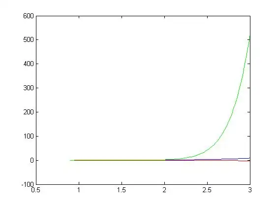
Plot

${\displaystyle y_{4}\!}$ shown in red

${\displaystyle y_{7}\!}$ shown in blue

${\displaystyle y_{11}\!}$ shown in green

Matlab Solution

The numerical solution calculated using the matlab ode45 command is shown below:

 ans =
   0.2788
   0.2854
   0.2923
   0.2997
   0.3074
   0.3229
   0.3401
   0.3592
   0.3804
   0.4040
   0.4302
   0.4595
   0.4921
   0.5285
   0.5691
   0.6145
   0.6651
   0.7218
   0.7850
   0.8557
   0.9346
   1.0228
   1.1213
   1.2313
   1.3542
   1.4914
   1.6445
   1.8155
   2.0063
   2.2193
   2.4569
   2.7219
   3.0175
   3.3471
   3.7146
   4.1243
   4.5809
   5.0898
   5.6568
   6.2885
   6.9921
   7.3442
   7.7142
   8.1032
   8.5119

Plot

Plotting the aboved vector of y-values,along with the results from earlier yields the following graph:

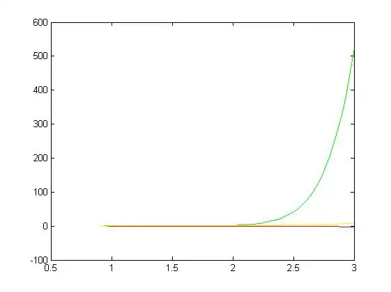
where the answer calculated in matlab is shown in yellow.

Egm4313.s12.team11.imponenti (talk) 08:04, 14 March 2012 (UTC)