University of Florida/Egm4313/s12.team5.R4

Report 4

R4.1

Question

For the series shown in the notes on p. 7-20

$\ \sum _{j=0}^{n-2}[c_{j+2}(j+2)(j+1)+ac_{j+1}(j+1)+bc_{j}]x^{j}+ac_{n}nx^{n-1}+b[c_{n-1}x^{n-1}+c_{n}x^{n}]=\sum _{j=0}^{n}d_{j}x^{j}\$

Obtain the equations for the coefficients of $\ x$ , $\ x^{2}$ , $\ x^{n-2}\$ , $\ x^{n-1}\$ , $\ x^{n}$

Then, set up the coefficient matrix A for the general case with the coefficients obtained.

Solution

For j=0:

 $\displaystyle 2c_{2}+ac_{1}+bc_{0}=d_{0}$   (1)

For j=1:

 $\displaystyle 6c_{3}+2ac_{2}+bc_{1}=d_{1}$   (2)

For j=2:

 $\displaystyle 12c_{4}+3ac_{3}+bc_{2}=d_{2}$  (3)

For j=n-2:

 $\displaystyle [c_{n}(n)(n-1)+ac_{n-1}(n-1)+bc_{n-2}]=d_{n-2}$  (4)

For j=n-1:

 $\displaystyle ac_{n}n+bc_{n-1}=d_{n-1}$  (5)

For j=n:

 $\displaystyle bc_{n}=d_{n}$  (6)

Setting up the A matrix using equations (1)-(6):

 $\displaystyle A={\begin{bmatrix}b&a&2&&&\\&b&2a&&&\\&&b&&&\\&&&b&a(n-1)&n(n-1)\\&&&&b&an\\&&&&&b\end{bmatrix}}$

Author

Solved and uploaded by Joshua House

Proofread by David Herrick

R 4.2

Question

Consider the L2-ODE-CC(5) p.7b-7 with sin x as excitation:

$\displaystyle \ y''-3y'+2y=r(x)\$

$\displaystyle \ r(x)=\sin x\$

and with the initial conditions $\displaystyle \ y(0)=1,y'(0)=0\$

Part 1

Use the Taylor series for $\displaystyle \ \sin x\$ in (1)p6-4 to reproduce the figure on p7-24

Part 2

Let $\displaystyle \ y_{p}(x)\$ be the particular soln corresponding to the excitating $\displaystyle \ r_{n}(x)\$ : $\displaystyle \ y''_{p}+ay'_{p}+by_{p}=r_{n}(x)\$

Let $\displaystyle \ r_{n}(x)\$ be the truncated Taylor series of sin x :

$\sum _{n=0}^{\infty }{\frac {(-1)^{k}(t)^{2k+1}}{(2k+1)!}}=t-{\frac {t^{3}}{3!}}+...+{\frac {(-1)^{n}(t)^{2n+1}}{(2n+1)!}}=:r_{n}(x)\$

Let $\ y_{n}(x)\$ be the overall soln for the L2-ODE-CC corresponding to (2)-(3) p.7-26 :

$\displaystyle \ y''_{n}+ay'_{n}+by_{n}=r_{n}(x)\$

with the same initial conditions (3b)p.3-7.

Find the $\ y_{n}(x)\$ for n = 3, 5, 9; plot these solns for x in the interval [0,4π].

Part 3

Use the particular soln in K 2011 p.82 Table 2.1 to find the exact overall soln y(x) and plot it in the above figure to compare with $\ y_{n}(x)\$ for n = 3, 5, 9.

Solution

Part 1

Part 2

To solve the non-homogeneous ODE we have to solve the homogeneous ODE and find any solution of $\ y_{p}(x)\$ . Using the method of undetermined coefficients, specifically the basic rule, where r(x) is in one of the functions in the first column in Table 2.1 K 2011 p. 82 and choose the $\ y_{p}(x)\$ in the same line and determine its undetermined coefficients by substituting $\ y_{p}\$ and its derivatives.

For an excitation $\ r_{n}(x)\$

n = 3

$\displaystyle \ r_{3}(x)=t-(t^{3})/3!\$

n = 5

$\displaystyle \ r_{5}(x)=t-(t^{3})/3!+(t^{5})/5!\$

n = 9

$\displaystyle \ r_{9}(x)=t-(t^{3})/3!+(t^{5})/5!-(t^{7})/7!+(t^{9})/9!\$

The term in $\ r(x)\$ that will be used will be $\ kx^{n}(n=3,5,9)\$

For n = 3

$\ K_{3}x^{3}+K_{2}x^{2}+K_{1}x+K_{0}\$

For n = 5

$\ K_{5}x^{5}+K_{4}x^{4}+K_{3}x^{3}+K_{2}x^{2}+K_{1}x+K_{0}\$

For n = 9

$\ K_{9}x^{9}+K_{8}x^{8}+K_{7}x^{7}+K_{6}x^{6}+K_{5}x^{5}+K_{4}x^{4}+K_{3}x^{3}+K_{2}x^{2}+K_{1}x+K_{0}\$

The homogeneous solution for y will be in the form of

$\displaystyle \ y_{h}(x)=C_{1}e^{2x}+C_{2}e^{x}\$

Plugging $\ y_{p}'',y_{p}',y_{p}\$ into the original equation will give the following:

For n = 3

$\ (6K_{3}x+2K_{2})-3(3K_{3}x^{2}+2K_{2}x+K_{1})+2(K_{3}x^{3}+K_{2}x^{2}+K_{1}x+K_{0})=x-(x^{3})/6!\$

For n = 5

$\ (20K_{5}x^{3}+12K_{4}x^{2}+6K_{3}x+4K_{2}x)-3(5K_{5}x^{4}+4K_{4}x^{3}+3K_{3}x^{2}+2K_{2}x+K_{1})+2(K_{5}x^{5}+K_{4}x^{4}+K_{3}x^{3}+K_{2}x^{2}+K_{1}x+K_{0})\$

$\ =x-(x^{3})/3!+(x^{5})/5!\$

For n = 9

$\ (72K_{9}x^{7}+56K_{8}x^{6}+42K_{7}x^{5}+30K_{6}x^{4}+20K_{5}x^{3}+12K_{4}x^{2}+6K_{3}x+4K_{2}x)-3(9K_{9}x^{8}+8K_{8}x^{7}+7K_{7}x^{6}+6K_{6}x^{5}+5K_{5}x^{4}+4K_{4}x^{3}\$

$\ +3K_{3}x^{2}+2K_{2}x+K_{1}+2(K_{9}x^{9}+K_{8}x^{8}+K_{7}x^{7}+K_{6}x^{6}+K_{5}x^{5}+K_{4}x^{4}+K_{3}x^{3}+K_{2}x^{2}+K_{1}x+K_{0})=x-(x^{3})/3!+(x^{5})/5!-(x^{7})/7!+(x^{9})/9!\$

Equating the coefficients of $\ x^{n}\$ on both sides

For n = 3

$\ x^{3}:2K_{3}=-1/6\$

$\ K_{3}=-1/12\$

$\ x^{2}:-9K_{3}+2K_{2}=0\$

$\ K_{2}=-3/8\$

$\ x:6K_{3}-6K_{2}+2K_{1}=1\$

$\ K_{1}=-3/8\$

$\ c:2K_{2}-3K_{1}+2K_{0}=0\$

$\ K_{0}=-3/16\$

Now plugging in the particular and homogeneous equation $\ y=y_{h}+y_{p}\$ and solving for the initial conditions.

$\ y=C_{1}e^{2x}+C_{2}e^{x}-(1/12)x^{3}-(3/8)x^{2}-(3/8)x-3/16\$ $\ y(0)=C_{1}+C_{2}-3/16=1\$ $\ y'(0)=2C_{1}+C_{2}-3/8=0\$

This gives constant values of $\ C_{1}=-13/16\$ $\ C_{2}=2\$

For n = 3 Final solution is:

$\ y_{3}=(-13/16)e^{2x}+2e^{x}-(1/12)x^{3}-(3/8)x^{2}-(3/8)x-3/16\$

For n = 5

Equating the coefficients

$\ x^{5}:2K_{5}=1/120\$

$\ K_{5}=1/240\$

$\ x^{4}:-15K_{5}+2K_{4}=0\$

$\ K_{4}=1/32\$

$\ x^{3}:20K_{5}-12K_{4}+2K_{3}=-1/6\$

$\ K_{3}=-11/24\$

$\ x^{2}:12K_{4}-9K_{3}+2K_{2}=0\$

$\ K_{2}=-9/4\$

$\ x:6K_{3}-6K_{2}+2K_{1}=1\$

$\ K_{1}=-39/8\$

$\ c:4k_{2}-3K_{1}+2K_{0}=0\$

$\ K_{0}=-45/16\$

Now plugging in the particular and homogeneous equation $\ y=y_{h}+y_{p}\$ and solving for the initial conditions.

$\ y=C_{1}e^{2x}+C_{2}e^{x}+(1/240)x^{5}+(1/32)x^{4}-(11/24)x^{3}-(9/4)x^{2}-(39/8)x-45/16\$

$\ y(0)=C_{1}+C_{2}-45/16=1\$

$\ y'(0)=2C_{1}+C_{2}-39/8=0\$

This gives constant values of $\ C_{1}=79/48\$ $\ C_{2}=13/6\$

For n = 5 the final solution is

$\ y_{5}=(79/48)e^{2x}+(13/6)e^{x}+(1/240)x^{5}+(1/32)x^{4}-(11/24)x^{3}-(9/4)x^{2}-(39/8)x-45/16\$

For n = 9

Equating the coefficients

$\ x^{9}:2K_{9}=1/9!\$

$\ K_{9}=1.3778e^{-6}\$

$\ x^{8}:-27K_{9}+2K_{8}=0\$

$\ k_{8}=1.86e^{-5}\$

$\ x^{7}:72K_{9}-24K_{8}+2K_{7}=-1/7!\$

$\ K_{7}=2.728e^{-4}\$

$\ x^{6}:56K_{8}-21K_{7}+2K_{6}=0\$

$\ K_{6}=0.0023\$

$\ x^{5}:42K_{7}-18K_{6}+2K_{5}=1/5!\$

$\ K_{5}=0.0111\$

$\ x^{4}:30K_{6}-15K_{5}+2K_{4}=0\$

$\ K_{4}=0.0488\$

$\ x^{3}:20K_{5}-12K_{4}+2K_{3}=-1/3!\$

$\ K_{3}=0.0976)\$

$\ x^{2}:12K_{4}-9K_{3}+2K_{2}=0\$

$\ K_{2}=0.1463\$

$\ x:6K_{3}-6K_{2}+2K_{1}=1\$

$\ K_{1}=0.6461\$

$\ c:4K_{2}-3K_{1}+2K_{0}=0\$

$\ K_{0}=0.6765\$

Now plugging in the particular and homogeneous equation $\ y=y_{h}+y_{p}\$ and solving for the initial conditions.

$\ y=C_{1}e^{2x}+C_{2}e^{x}+y_{p}\$

$\ y(0)=C_{1}+C_{2}+0.6765=1\$

$\ y'(0)=2C_{1}+C_{2}+0.6461=0\$

This gives constant values of

$\ C_{1}=-0.3226\$

$\ C_{2}=0.6449\$

For n = 9 the final solution is

$\ y_{9}=-0.3226e^{2x}+0.6449e^{x}+1.37e^{-6}x^{9}+1.86e^{-5}x^{8}+2.72e^{-4}x^{7}+0.0023x^{6}+0.0111x^{5}+0.0488x^{4}-0.0976x^{3}\$

$\ -0.1463x^{2}-0.6461x-0.6765\$

Part 3

The table 2.1 from K 2011 p.82 illustrates that for the method of undetermined coefficients for an r(x) term in the form of:

r(x) = k sin(ωx)

Then the choice for $\ y_{p}(x)\$ would be:

K cos(ωx) + M sin(ωx)

The homogeneous solution for y will be in the form of

$\displaystyle \ y_{h}(x)=y(x)=C_{1}e^{2x}+C_{2}e^{x}\$

with roots of 2 and 1 derived from $\displaystyle \ y''-3y'+2y=0\$

Plugging in the derivatives for the particular solution into the original equation gives:

$\displaystyle \ y_{p}''-3y_{p}'+2y_{p}=sin(x)\$

where

      $\ y_{p}=Acos(x)+Bsin(x)\$

      $\ y_{p}'=-Asin(x)+Bcos(x)\$

      $\ y_{p}''=-Acos(x)-Bsin(x)\$

      $\displaystyle \ -Acos(x)-Bsin(x)-3(-Asin(x)+Bcos(x))+2(Acos(x)+Bsin(x))=sin(x)\$

      $\displaystyle \ (A-3B)cos(x)+(3A+B)sin(x)=sin(x)\$

      $\ 3A+B=1;A-3B=0;\$

      $\ A=3/10;B=1/10\$

Combining the particular and homogeneous solution of y gives the following:

$\displaystyle \ y=y_{h}+y_{p}=C_{1}e^{2x}+C_{2}e^{x}+(3/10)cos(x)+(1/10)sin(x)\$

Solving for the initial conditions where $\ y(0)=1,andy'(0)=0\$

$\ y(0)=C_{1}+C_{2}=7/10\$

$\ y'(0)=2C_{1}+C_{2}+1/10\$

$\ 2C_{1}+7/10-C_{1}=-1/10\$

$\ C_{1}=-8/10;C_{2}=-1/10\$

This gives the final solution:

$\displaystyle \ y=(-8/10)e^{2x}-(1/10)e^{x}+(3/10)cos(x)+(1/10)sin(x)\$

From the figure it is barely discernible between this figure and the figure above it in part two. The final solution for y in part three is very similar if not approximately identical to the lower curve in the figure in part two.

Author

This problem was solved and uploaded by Michael Wallace

R 4.3

Question

Consider the L2-ODE-CC:

$\displaystyle \ y''-3y'+2y=r(x)\$

Where $\displaystyle \ r(x)=\log(1+x)\$

with initial conditions $\displaystyle \ y(-{\frac {3}{4}})=1,y'(-{\frac {3}{4}})=0\$

Part 1

Develop $\displaystyle \ \log(1+x)\$ in Taylor series about x(hat) = 0 to reproduce the figure in the notes on p. 7-25.

Part 2

Let $\displaystyle \ r_{n}(x)\$ be the truncated Taylor series with n terms -- which is also the highest degree of the Taylor (power) series -- of $\displaystyle \ \log(1+x)\$ .

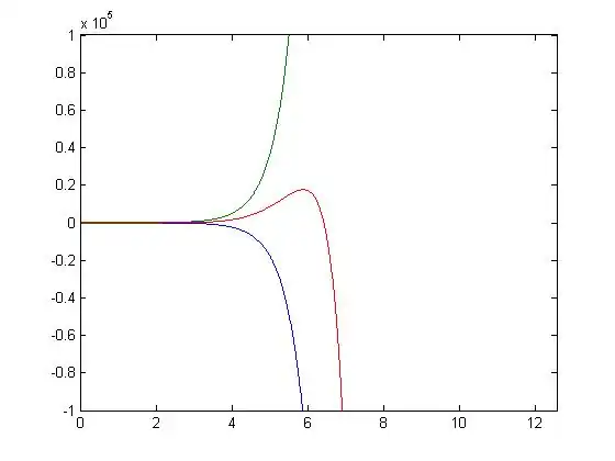
Find $\displaystyle \ y_{n}(x)\$ for n = 4, 7, and 11 such that:

$\displaystyle \ y_{n}''+ay_{n}'+by_{n}=r_{n}(x)\$

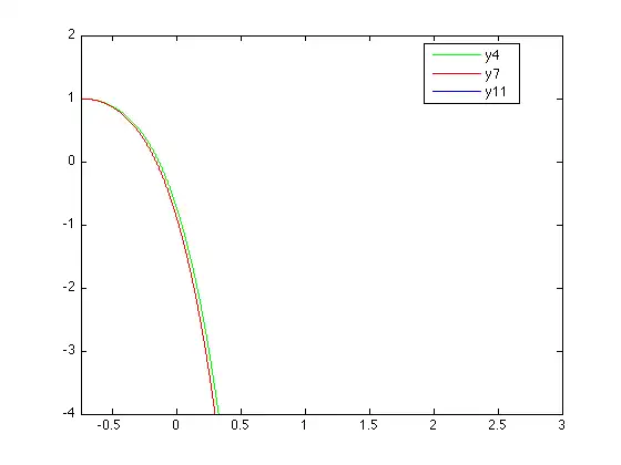
Plot $\displaystyle \ y_{n}(x)\$ for n = 4,7,11 for x in $\displaystyle \ [-{\frac {3}{4}},3]\$

Part 3

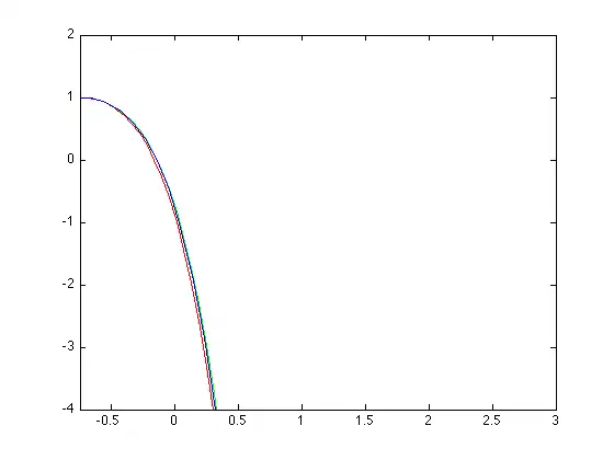
Use the matlab command ODE45 to integrate numerically the same function with the same initial conditions to obtain $\displaystyle \ y(x)\$ . Then plot $\displaystyle \ y(x)\$ in the same figure with $\displaystyle \ y_{n}(x)\$

Solution

Part 1

The formula to develop the Taylor Series about x(hat) = 0 is given by:

$\displaystyle \ f(0)+{\frac {f'(0)(x-0)^{1}}{1!}}+{\frac {f''(0)(x-0)^{2}}{2!}}+{\frac {f'''(0)(x-0)^{3}}{3!}}+...\sum _{n=0}^{\infty }{\frac {f^{n}(0)(x-0)^{n}}{n!}}\$

Using the function $\displaystyle \ \log(1+x)\$ we get:

$\displaystyle \ f'(x)={\frac {1}{(x+1)}},f''(x)={\frac {-1}{(x+1)^{2}}},f'''(x)={\frac {2}{(x+1)^{3}}},...\$

Plugging in 0, the first few terms become:

$\displaystyle \ 0+x-{\frac {x^{2}}{2}}+{\frac {x^{3}}{3}}\$

The pattern of this expression can be represented by the Taylor series:

 $\sum _{n=0}^{\infty }{\frac {(-1)^{n}(x)^{n+1}}{(n+1)}}$

Part 2

First, the homogenous solution to the differential equation is given by:

$\displaystyle \ (\lambda -1)(\lambda -2)=0\$

Therefore, $\displaystyle \ y_{h}=C_{1}e^{x}+C_{2}e^{2x}\$

for $\displaystyle \ r_{n}(x)\$ is given by the truncated Taylor series of 4 terms:

$\displaystyle \ r_{4}(x)=x-{\frac {x^{2}}{2}}+{\frac {x^{3}}{3}}-{\frac {x^{4}}{4}}\$

Therefore, $\displaystyle \ y_{p4}=c_{0}+c_{1}x+c_{2}x^{2}+c_{3}x^{3}+c_{4}x^{4}\$

$\displaystyle \ y_{p4}'=c_{1}+2c_{2}x+3c_{3}x^{2}+4c_{4}x^{3},y_{p4}''=2c_{2}+6c_{3}x+12c_{4}x^{2}\$

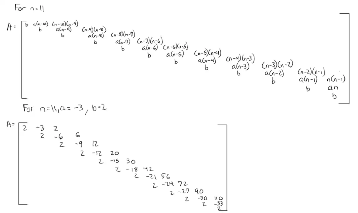
For this solution, with n = 4, the coefficient matrix is set up like:

$\displaystyle \ A={\begin{bmatrix}b&a(n-3)&(n-3)(n-2)&&\\&b&a(n-2)&(n-1)(n-2)&\\&&b&a(n-1)&n(n-1)\\&&&b&an\\&&&&b\end{bmatrix}}\$

Therefore, the matrix solution with n = 4, a = -3, and b = 2 is:

$\displaystyle \ A={\begin{bmatrix}2&-3&2&&\\&2&-6&6&\\&&2&-9&12\\&&&2&-12\\&&&&2\end{bmatrix}}{\begin{bmatrix}c_{0}\\c_{1}\\c_{2}\\c_{3}\\c_{4}\end{bmatrix}}={\begin{bmatrix}0\\1\\-{\frac {1}{2}}\\{\frac {1}{3}}\\-{\frac {1}{4}}\end{bmatrix}}\$

Solving by back substitution we get:

$\displaystyle \ y_{p4}=-{\frac {65}{16}}-{\frac {33}{8}}x-{\frac {17}{8}}x^{2}-{\frac {7}{12}}x^{3}-{\frac {1}{8}}x^{4}\$

$\displaystyle \ y_{4}(x)=C_{1}e^{x}+C_{2}e^{2x}-{\frac {65}{16}}-{\frac {33}{8}}x-{\frac {17}{8}}x^{2}-{\frac {7}{12}}x^{3}-{\frac {1}{8}}x^{4}\$

Plugging in the initial conditions we get:

 $\displaystyle \ y_{4}(x)=8.90e^{x}-5.587e^{2x}-{\frac {65}{16}}-{\frac {33}{8}}x-{\frac {17}{8}}x^{2}-{\frac {7}{12}}x^{3}-{\frac {1}{8}}x^{4}\$

for $\displaystyle \ r_{n}(x)\$ is given by the truncated Taylor series of 7 terms:

$\displaystyle \ r_{7}(x)=x-{\frac {x^{2}}{2}}+{\frac {x^{3}}{3}}-{\frac {x^{4}}{4}}+{\frac {x^{5}}{5}}-{\frac {x^{6}}{6}}+{\frac {x^{7}}{7}}\$

Therefore: $\displaystyle \ y_{p7}=c_{0}+c_{1}x+c_{2}x^{2}+c_{3}x^{3}+c_{4}x^{4}+c_{5}x^{5}+c_{6}x^{6}+c_{7}x^{7}\$

$\displaystyle \ y_{p7}'=c_{1}+2c_{2}x+3c_{3}x^{2}+4c_{4}x^{3}+5c_{5}x^{4}+6c_{6}x^{5}+7c_{7}x^{6}\$

$\displaystyle \ y_{p7}''=2c_{2}+6c_{3}x+12c_{4}x^{2}+20c_{5}x^{3}+30c_{6}x^{4}+42c_{7}x^{5}\$

For this solution, with n = 7, the coefficient matrix is set up like:

$\displaystyle \ A={\begin{bmatrix}b&a(n-6)&(n-6)(n-5)&&&&&\\&b&a(n-5)&(n-5)(n-4)&&&&\\&&b&a(n-4)&(n-4)(n-3)&&&\\&&&b&a(n-3)&(n-3)(n-2)&&\\&&&&b&a(n-2)&(n-2)(n-1)&\\&&&&&b&a(n-1)&(n-1)(n)\\&&&&&&b&an\\&&&&&&&b\end{bmatrix}}\$

Therefore, the matrix solution with n = 7, a = -3, and b = 2 is:

$\displaystyle \ A={\begin{bmatrix}2&-3&2&&&&&\\&2&-6&6&&&&\\&&2&-9&12&&&\\&&&2&-12&20&&\\&&&&2&-15&30&\\&&&&&2&-18&42\\&&&&&&2&-21\\&&&&&&&2\end{bmatrix}}{\begin{bmatrix}c_{0}\\c_{1}\\c_{2}\\c_{3}\\c_{4}\\c_{5}\\c_{6}\\c_{7}\end{bmatrix}}={\begin{bmatrix}0\\1\\-{\frac {1}{2}}\\{\frac {1}{3}}\\-{\frac {1}{4}}\\{\frac {1}{5}}\\-{\frac {1}{6}}\\{\frac {1}{7}}\end{bmatrix}}\$

Solving by back substitution we get:

$\displaystyle \ y_{p7}={\frac {49317}{80}}+{\frac {24573}{40}}x+{\frac {12201}{40}}x^{2}+{\frac {1205}{12}}x^{3}+{\frac {195}{8}}x^{4}+{\frac {23}{5}}x^{5}+{\frac {2}{3}}x^{6}+{\frac {1}{14}}x^{7}\$

Since the homogeneous solution remains the same:

$\displaystyle \ y_{7}(x)=C_{1}e^{x}+C_{2}e^{2x}+{\frac {49317}{80}}+{\frac {24573}{40}}x+{\frac {12201}{40}}x^{2}+{\frac {1205}{12}}x^{3}+{\frac {195}{8}}x^{4}+{\frac {23}{5}}x^{5}+{\frac {2}{3}}x^{6}+{\frac {1}{14}}x^{7}\$

Plugging in the initial conditions we get:

 $\displaystyle \ y_{7}(x)=-613.504e^{x}-3.868e^{2x}+{\frac {49317}{80}}+{\frac {24573}{40}}x+{\frac {12201}{40}}x^{2}+{\frac {1205}{12}}x^{3}+{\frac {195}{8}}x^{4}+{\frac {23}{5}}x^{5}+{\frac {2}{3}}x^{6}+{\frac {1}{14}}x^{7}\$

The image below demonstrates the general matrix for n=11 and the matrix with values filled in:

for $\displaystyle \ r_{n}(x)\$ is given by the truncated Taylor series of 11 terms:

$\displaystyle \ r_{11}(x)=x-{\frac {x^{2}}{2}}+{\frac {x^{3}}{3}}-{\frac {x^{4}}{4}}+{\frac {x^{5}}{5}}-{\frac {x^{6}}{6}}+{\frac {x^{7}}{7}}-{\frac {x^{8}}{8}}+{\frac {x^{9}}{9}}-{\frac {x^{10}}{10}}+{\frac {x^{11}}{11}}\$

Therefore, $\displaystyle \ y_{p11}=c_{0}+c_{1}x+c_{2}x^{2}+c_{3}x^{3}+c_{4}x^{4}+c_{5}x^{5}+c_{6}x^{6}+c_{7}x^{7}+c_{8}x^{8}+c_{9}x^{9}+c_{10}x^{10}+c_{11}x^{11}$

Solving by back substitution we get:

$\ y_{p11}=3301079.406+3300338.812x+1649428.813x^{2}+549316.042x^{3}+137082.188x^{4}+27317.725x^{5}+4520.042x^{6}$

$\ +636.321x^{7}+77.188x^{8}+8.056x^{9}+0.7x^{10}+0.0455x^{11}$

Since the homogeneous solution remains the same:

$\ y_{11}(x)=C_{1}e^{x}+C_{2}e^{2x}+3301079.406+3300338.812x+1649428.813x^{2}+549316.042x^{3}+137082.188x^{4}+27317.725x^{5}+4520.042x^{6}$

$\ +636.321x^{7}+77.188x^{8}+8.056x^{9}+0.7x^{10}+0.0455x^{11}\$

Plugging in the initial conditions we get:

 $\ y_{11}(x)=-3391815.1e^{x}+734.909e^{2x}+3301079.406+3300338.812x+1649428.813x^{2}+549316.042x^{3}+137082.188x^{4}+27317.725x^{5}\$

 $\ +4520.042x^{6}+636.321x^{7}+77.188x^{8}+8.056x^{9}+0.7x^{10}+0.0455x^{11}\$

Part 3

Matlab Code:

function yp = F(t,y)

yp = zeros(2,1);

yp(1) = y(2);

yp(2) = log(t+1) + 3*y(2)-2*y(1);

end

[t,y] = ode45('F',[-.75,3],[1,0]);

plot(x,y4,'g',x,y7,'r',x,y11,'y',t,y(:,1),'b')

axis([-0.75 3 -4 2])

Author

Part 2 n=7 and n =11 were solved and uploaded by Cameron North.

Part 1 and Part 2 n = 4 was solved and uploaded by David Herrick

R 4.4

Question

Part 1

Find n sufficiently high so that $y_{n}(x_{1}),y'_{n}(x_{1})$ do not differ from the numerical solution by more than $10^{-5}$ at $x_{1}=0.9$

Part 2

Develop log(1+x) in Taylor series about ${\hat {x}}=1$ . Plot the results.

Part 3

Find $y_{n}(x)$ for n=4,7,11, such that $y_{n}''+ay_{n}'+by_{n}=r_{n}(x)$ for x in [0.9,3] with the initial conditions found in Part 1. Plot the results.

Part 4

Use the matlab command 'ode45' to integrate numerically (5) p.7b-7 with (1) p.7-28 and the initial conditions $\displaystyle y_{n}(x_{1}),y'_{n}(x_{1})$ to obtain the numerical solution for $\displaystyle y(x)$ .
Plot $\displaystyle y(x)$ in the same figure with $\displaystyle y_{n}(x)$

Solution

Part 1

With MATLAB, a program was used to iteratively add terms into the taylor series of $log(1+x)$ . Until the error between the exact answer and the series was less than $10^{-5}$ ., more terms were added.

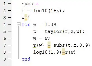
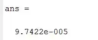
$n=39$ for the error to be of a magnitude of $10^{-5}$ . The error found: 9.7422e-005

With a very similar process for $y'_{n}(x_{1})$ .

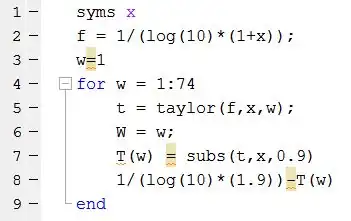
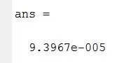
$n=74$ for the error to be of a magnitude of $10^{-5}$ . The error found: 9.3967e-005

Part 2

The formula to develop the Taylor Series about ${\hat {x}}=1$ is given by:

$\displaystyle \ f(1)+{\frac {f'(1)(x-1)^{1}}{1!}}+{\frac {f''(1)(x-1)^{2}}{2!}}+{\frac {f'''(1)(x-1)^{3}}{3!}}+...\sum _{n=0}^{\infty }{\frac {f^{n}(1)(x-1)^{n}}{n!}}\$

Using the function $\displaystyle \ \log(1+x)\$ for n=11 we get:

$\displaystyle \ f'(x)={\frac {1}{(x+1)}},f''(x)={\frac {-1}{(x+1)^{2}}},f'''(x)={\frac {2}{(x+1)^{3}}},f^{IV}(x)={\frac {-6}{(x+1)^{4}}},\$
$\displaystyle \ f^{V}(x)={\frac {24}{(x+1)^{5}}},f^{VI}(x)={\frac {-120}{(x+1)^{6}}},f^{VII}(x)={\frac {720}{(x+1)^{7}}},f^{VIII}(x)={\frac {-5040}{(x+1)^{8}}},\$
$\displaystyle \ f'^{X}(x)={\frac {40320}{(x+1)^{9}}},f^{X}(x)={\frac {-362880}{(x+1)^{10}}},f^{XI}(x)={\frac {3628800}{(x+1)^{11}}}\$

Plugging in x=1 up to n=4, and using the formula for developing the Taylor Series, we get $y_{n4}$ :

 $\displaystyle \ y_{n4}=log(2)+{\frac {(x-1)}{2}}-{\frac {(x-1)^{2}}{8}}+{\frac {(x-1)^{3}}{24}}-{\frac {(x-1)^{4}}{64}}\$ ,

Then we do the same for n=7 terms to get $y_{n7}$ :

 $\displaystyle \ y_{n7}=log(2)+{\frac {(x-1)}{2}}-{\frac {(x-1)^{2}}{8}}+{\frac {(x-1)^{3}}{24}}-{\frac {(x-1)^{4}}{64}}+{\frac {(x-1)^{5}}{160}}-{\frac {(x-1)^{6}}{384}}+{\frac {(x-1)^{7}}{896}}\$

And finally for $y_{n11}$ :

 $\displaystyle \ y_{n11}=log(2)+{\frac {(x-1)}{2}}-{\frac {(x-1)^{2}}{8}}+{\frac {(x-1)^{3}}{24}}-{\frac {(x-1)^{4}}{64}}+{\frac {(x-1)^{5}}{160}}-{\frac {(x-1)^{6}}{384}}+{\frac {(x-1)^{7}}{896}}-{\frac {(x-1)^{8}}{2048}}+{\frac {(x-1)^{9}}{4608}}-{\frac {(x-1)^{10}}{10240}}\ +{\frac {(x-1)^{11}}{22528}}$

Plotting the functions:
Matlab code:

x=-3:0.2:6;
y = log(1+x);
y4 = log(2) + (x-1)/2 - (x-1).^2/8 + (x-1).^3/24 - (x-1).^4/64;
y7 = log(2) + (x-1)/2 - (x-1).^2/8 + (x-1).^3/24 - (x-1).^4/64 + (x-1).^5/160 - (x-1).^6/384 + (x-1).^7/896;
y11 = log(2) + (x-1)/2 - (x-1).^2/8 + (x-1).^3/24 - (x-1).^4/64 + (x-1).^5/160 - (x-1).^6/384 + (x-1).^7/896 - (x-1).^8/2048 + (x-1).^9/4608 - (x-1).^(10)/10240 + (x-1).^(11)/22528;
plot(x,y, x,y4, x,y7, x,y11)
hleg1 = legend('log(1+x)','n=4','n=7','n=11');

Graph:

Convergence is in the domain [-1.5,4].

Part3

For n=4 $r_{x}$ is:

 $\displaystyle \ r_{x}=log(2)+{\frac {(x-1)}{2}}-{\frac {(x-1)^{2}}{8}}+{\frac {(x-1)^{3}}{24}}-{\frac {(x-1)^{4}}{64}}\$

$\displaystyle \ y_{p4}=c_{0}+c_{1}(x-1)-c_{2}(x-1)^{2}+c_{3}(x-1)^{3}-c_{4}(x-1)^{4}\$
$\displaystyle \ y_{n4}'=c_{1}-2c_{2}(x-1)+3c_{3}(x-1)^{2}-4c_{4}(x-1)^{3}\$
$\displaystyle \ y_{n4}''=-2c_{2}+6c_{3}(x-1)-12c_{4}(x-1)^{2}\$ ,

Plugging the equations into the above ODE will give matrices like the following:

{\begin{bmatrix}2&0&0&0&0\\-12&2&0&0&0\\12&-9&2&0&0\\0&6&-6&2&0\\0&0&2&-3&2\end{bmatrix}}*{\begin{bmatrix}c_{4}\\c_{3}\\c_{2}\\c_{1}\\c_{0}\end{bmatrix}}={\begin{bmatrix}-{\frac {1}{64ln(10)}}\\{\frac {1}{24ln(10)}}\\-{\frac {1}{8ln(10)}}\\{\frac {1}{2ln(10)}}\\log(2)\end{bmatrix}}\!

The unknown vector $c\!$ can be solved by forward substitution, with MATLAB to do the calculations:

$c_{4}=-.0034,c_{3}=-.0113,c_{2}=-.0577,c_{1}=-.1624,c_{0}=.1624\!$

Particular and general solution $y_{p4}\!$ , $y_{4}\!$ :

$y_{p4}=0.1624-0.1624*(x-1)-.0577*(x-1)^{2}-.0113*(x-1)^{3}-.0034*(x-1)^{4}\!$

$y_{4}(x)=y_{h}(x)+y_{p4}(x)\!$

$y_{4}(x)=C_{1}e^{x}+C_{2}e^{2x}+0.1624-0.1624*(x-1)\!$ $-.0577*(x-1)^{2}-.0113*(x-1)^{3}-.0034*(x-1)^{4}\!$

Then with the Initial Conditions,

 $y_{4}(x)=.0595e^{x}-.0076e^{2x}+0.1624-0.1624*(x-1)\!$ 
 $-.0577*(x-1)^{2}-.0113*(x-1)^{3}-.0034*(x-1)^{4}\!$

For n=7 $r_{x}$ is:

 $\displaystyle \ r_{x}=log(2)+{\frac {(x-1)}{2}}-{\frac {(x-1)^{2}}{8}}+{\frac {(x-1)^{3}}{24}}-{\frac {(x-1)^{4}}{64}}+{\frac {(x-1)^{5}}{160}}-{\frac {(x-1)^{6}}{384}}+{\frac {(x-1)^{7}}{896}}\$

$\displaystyle \ y_{p7}=c_{0}+c_{1}(x-1)-c_{2}(x-1)^{2}+c_{3}(x-1)^{3}-c_{4}(x-1)^{4}+c_{5}(x-1)^{5}-c_{6}(x-1)^{6}+c_{7}(x-1)^{7}\$

$\displaystyle \ y_{p7}'=c_{1}-2c_{2}(x-1)+3c_{3}(x-1)^{2}-4c_{4}(x-1)^{3}+5c_{5}(x-1)^{4}-6c_{6}(x-1)^{5}+7c_{7}(x-1)^{6}\$

$\displaystyle \ y_{p7}''=-2c_{2}+6c_{3}(x-1)-12c_{4}(x-1)^{2}+20c_{5}(x-1)^{3}-30c_{6}(x-1)^{4}+42c_{7}(x-1)^{5}\$

The same process used when solving when n=4 is used to construct a matrix equation for n=7:

{\begin{bmatrix}2&0&0&0&0&0&0&0\\-21&2&0&0&0&0&0&0\\42&-18&2&0&0&0&0&0\\0&30&-15&2&0&0&0&0\\0&0&20&-12&2&0&0&0\\0&0&0&12&-9&2&0&0\\0&0&0&0&6&-6&2&0\\0&0&0&0&0&2&-3&2\end{bmatrix}}*{\begin{bmatrix}c_{7}\\c_{6}\\c_{5}\\c_{4}\\c_{3}\\c_{2}\\c_{1}\\c_{0}\end{bmatrix}}={\begin{bmatrix}{\frac {1}{896ln(10)}}\\-{\frac {1}{384ln(10)}}\\{\frac {1}{160ln(10)}}\\-{\frac {1}{64ln(10)}}\\{\frac {1}{24ln(10)}}\\-{\frac {1}{8ln(10)}}\\{\frac {1}{2ln(10)}}\\log(2)\end{bmatrix}}\!

Using MATLAB to solve for the unknown vector $c\!$ :

$c_{7}=.0002,c_{6}=.0020,c_{5}=.0141,c_{4}=.0725,c_{3}=.3034,c_{2}=.9029,c_{1}=1.9072,c_{0}=2.1084\!$

Particular and general solutions $y_{p7}\!$ , $y_{7}\!$ :

$y_{p7}=2.1084+1.9072*(x-1)+.9029*(x-1)^{2}+.3034*(x-1)^{3}+.0725*(x-1)^{4}+.0141*(x-1)^{5}+.0020*(x-1)^{6}+.0002*(x-1)^{7}\!$

$y_{7}(x)=y_{h}(x)+y_{p7}(x)\!$

$y_{7}(x)=C_{1}e^{x}+C_{2}e^{2x}+2.1084+1.9072*(x-1)+.9029*(x-1)^{2}+.3034*(x-1)^{3}+.0725*(x-1)^{4}+.0141*(x-1)^{5}\!$

$+.0020*(x-1)^{6}+.0002*(x-1)^{7}\!$

With the initial conditions:

 $y_{7}(x)=-.7271e^{x}+.0233e^{2x}+2.1084+1.9072*(x-1)+.9029*(x-1)^{2}+.3034*(x-1)^{3}+.0725*(x-1)^{4}+.0141*(x-1)^{5}!$

 $+.0020*(x-1)^{6}+.0002*(x-1)^{7}\!$

For n=11 $r_{x}$ is:

 $\displaystyle \ r_{x}=log(2)+{\frac {(x-1)}{2}}-{\frac {(x-1)^{2}}{8}}+{\frac {(x-1)^{3}}{24}}-{\frac {(x-1)^{4}}{64}}+{\frac {(x-1)^{5}}{160}}-{\frac {(x-1)^{6}}{384}}+{\frac {(x-1)^{7}}{896}}-{\frac {(x-1)^{8}}{2048}}+{\frac {(x-1)^{9}}{4608}}-{\frac {(x-1)^{10}}{10240}}\ +{\frac {(x-1)^{11}}{22528}}\$

$\displaystyle \ y_{p11}=c_{0}+c_{1}(x-1)-c_{2}(x-1)^{2}+c_{3}(x-1)^{3}-c_{4}(x-1)^{4}+c_{5}(x-1)^{5}-c_{6}(x-1)^{6}+c_{7}(x-1)^{7}-(x-1)^{8}+(x-1)^{9}-(x-1)^{10}+(x-1)^{11}\$ $\displaystyle \ y_{p11}'=c_{1}-2c_{2}(x-1)+3c_{3}(x-1)^{2}-4c_{4}(x-1)^{3}+5c_{5}(x-1)^{4}-6c_{6}(x-1)^{5}+7c_{7}(x-1)^{6}\$

$\displaystyle \ -8c_{8}(x-1)^{7}+9c_{9}(x-1)^{8}-10c_{10}(x-1)^{9}+11c_{11}(x-1)^{10}\$ $\displaystyle \ y_{p11}''=-2c_{2}+6c_{3}(x-1)-12c_{4}(x-1)^{2}+20c_{5}(x-1)^{3}-30c_{6}(x-1)^{4}+42c_{7}(x-1)^{5}-56c_{8}(x-1)^{6}\$

$\displaystyle \ +72c_{9}(x-1)^{7}-90c_{10}(x-1)^{8}+110c_{11}(x-1)^{9}\$

Creating another matrix system and solving for the unknown vector $c\!$ :

$c_{11}=0,c_{10}=.0002,c_{9}=.0019,c_{8}=.0181,c_{7}=.15,c_{6}=1.0675,c_{5}=6.4597,\!$

$c_{4}=32.4318,c_{3}=130.0033,c_{2}=390.3968,c_{1}=781.289,c_{0}=781.6873\!$

Particular and general solutions $y_{p11}\!$ , $y_{1}1(x)\!$ :

$y_{p11}=781.6873+781.289*(x-1)+390.3968*(x-1)^{2}+130.0033*(x-1)^{3}+32.4318*(x-1)^{4}+\!$

$6.4597*(x-1)^{5}+1.0675*(x-1)^{6}+.15*(x-1)^{7}+.0181*(x-1)^{8}+.0019*(x-1)^{9}+.0002*(x-1)^{10}\!$

$y_{11}(x)=y_{h}(x)+y_{p11}(x)\!$

$y_{11}(x)=C_{1}e^{x}+C_{2}e^{2x}+781.6873+781.289*(x-1)\!$

$+390.3968*(x-1)^{2}+130.0033*(x-1)^{3}+32.4318*(x-1)^{4}\!$

$6.4597*(x-1)^{5}+1.0675*(x-1)^{6}+.15*(x-1)^{7}+.0181*(x-1)^{8}+.0019*(x-1)^{9}+.0002*(x-1)^{10}\!$

With initial conditions:

 $y_{11}(x)=-287.5907e^{x}+.05e^{2x}+781.6873+781.289*(x-1)+390.3968*(x-1)^{2}+130.0033*(x-1)^{3}+32.4318*(x-1)^{4}\!$

 $6.4597*(x-1)^{5}+1.0675*(x-1)^{6}+.15*(x-1)^{7}+.0181*(x-1)^{8}+.0019*(x-1)^{9}+.0002*(x-1)^{10}\!$

plot:

Part 4

The initial condition equation is:

$\displaystyle y''-3y'+2y=ln(1+x)$

The initial conditions are:

$\displaystyle y(0)=39,y'(0)=74$

To solve the problem, we first convert the 2nd order differential equation into two 1st order differential equations. The initial 2nd order then turns into these two equations:

$\displaystyle y_{1}=y,y_{2}=y'$

Taking the derivatives, we find that:

$\displaystyle y'_{1}=y_{2},y'_{2}=-2y_{1}-3y_{2}+ln(1+x)$

with the new initial conditions as:

$\displaystyle y_{1}(t_{0})=1,y_{2}(t_{0})=0,t_{0}={\frac {-3}{4}}$

Now, we create a MATLAB function, "F", that will return a vector-valued function. We do this with the following function:

function yp=F(x,y)
yp=zeros(2,1);
yp(1)=y(2);
yp(2)=-2*y(1)-3*y(2)+log(1+x);

We now incorporate the function into a simple MATLAB program which will calculate the results:

EDU>> [x,y]=ode45('F',[0,5],[39,74]);
EDU>> plot(y(:,1),y(:,2))

This generates the following graph of $\displaystyle y_{n}(x)$ :

Now we solve the initial value problem by hand to find y(x):

$\displaystyle y''-3y'+2y=ln(1+x)$

First, convert to the characteristic equation:

$\displaystyle \lambda ^{2}-3\lambda +2=0$
$\displaystyle \lambda _{1}=2,\lambda _{2}=1$
$\displaystyle y_{h}(x)=C_{1}e^{x}+C_{2}e^{2}x$

The excitation factor of ln(1+x) does not yield any useful value for $\displaystyle y_{p}(x)$ since the integral is nonelementary. Therefore, the final solution for y(x) with what is know is simply:

$\displaystyle y(x)=C_{1}e^{x}+C_{2}e^{2}x,y'(x)=C_{1}e^{x}+2C_{2}e^{2}x$ $\displaystyle y(0)=39,C_{1}+C_{2}=39$
$\displaystyle y'(0)=74,C_{1}+2C_{2}=74$
$\displaystyle C_{1}=4,C_{2}=35$
$\displaystyle y(x)=4e^{x}+35e^{2x}$

Graphing both solutions on the same graph yields the following:

MATLAB code: EDU>> z = 4*exp(x) + 25*exp(2*x)
plot(y(:,1),y(:,2),y(:,1),z)

Author

Contribution Summary

Problem 1 was solved and uploaded by Joshua House 15:34, 13 March 2012 (UTC)

Problem 2 was solved by Mike Wallace

Problem 3 part 2 was solved by John North and parts 1 and 3 were solved by David Herrick

Problem 4 part 1 and part of part3 were solved and uploaded by Derik Bell, parts 2 and 3 were solved by Radina Dikova, and part 4 was solved by William Knapper

This article is issued from Wikiversity. The text is licensed under Creative Commons - Attribution - Sharealike. Additional terms may apply for the media files.