University of Florida/Egm6341/s10.Team2/HW5
Problem 1: Determination of leading coefficients of polynomials
Statement
To show that the value of the constants and in the polynomials and


Solution
From page 26-2, we know that:

We select such that it is a odd function and


Therefore, using , we get:


(1)

Similarly, using , we get:


(2)

Author
Egm6341.s10.team2.lee 08:58, 24 March 2010 (UTC)
proofread --Egm6341.s10.team2.niki 14:53, 24 March 2010 (UTC)
Problem 2: Continuation of proof of trapezoidal error
Statement
Continue the proof of Trapezoidal Rule Error to steps 4a and 4b and determine and


Solution
From steps 3a and 3b( P.26-3) we get the expression
(P.26-3)
![{\displaystyle \displaystyle {\boldsymbol {E=[P_{2}(t)g^{(1)}(t)+P_{4}(t)g^{(3)}(t)]_{-1}^{+1}-\underbrace {\int _{-1}^{+1}P_{5}(t)g^{(5)}(t)dt} _{D}}}}](../../../../I/f05afbde2f04704b76067518a639169b2a054390.svg)
(P.26-3)


Step 4a
![{\displaystyle \displaystyle \int _{-1}^{+1}\underbrace {P_{5}(t)} _{v'}\underbrace {g^{(5)}(t)} _{u}dt=[g^{(5)}(t)P_{6}(t)]_{-1}^{+1}-\underbrace {\int _{-1}^{+1}[{P_{6}(t)g^{(6)}(t)}} _{E}]dt}](../../../../I/15ab1895cdc848658ce1640bbc292a68be63d20e.svg)
where,


Step 4b
![{\displaystyle \displaystyle \int _{-1}^{+1}[{\underbrace {P_{6}(t)} _{v'}\underbrace {g^{(6)}(t)} _{u}}]dt=E=[g^{(6)}(t)P_{7}(t)]_{-1}^{+1}-\int _{-1}^{+1}P_{7}(t)g^{(7)}(t)dt}](../../../../I/bbc1e5d1cd540e678f1b6002c9c56d4d5ba9efb7.svg)
where,


Selecting such that

,we get


Summary


Author
--Egm6341.s10.team2.niki 22:04, 23 March 2010 (UTC)
--Proofread by Egm6341.s10.team2.lee 10:14, 26 March 2010 (UTC)
Problem 3: Expression of as function of


Statement
find on P. 27-1

Solution
From Page 27-1, we know:

Now rearranging the terms on both sides to write in terms of , we get:
where the size of the interval,


It can also be easily verified by substituting which yields


Also when yields


Author
Srikanth Madala (SM)
Problem 4: Evaluation of which can be used to calculate the coefficients of the even power euler-maclaurin error series for trapezoidal rule

Statement
Find the values of and


Clue: Use the formula:

Solution
We know from the formula:
From Mtg 26,slide 26-1, we know the formula:


(1)

From Mtg 26,slide 26-3, we know the formula:


(2)

From problem 2 on this HW , where we deduced that:


(3)

Author
--Srikanth Madala 01:44, 24 March 2010 (UTC) Srikanth Madala (SM)
Problem 5: Derivation of the Error of the Trapezoidal Rule
Statement
P. 28-2 derive
Derive the Following Equation for the error of the trapezoidal rule:
![{\displaystyle E_{n}^{1}=I-T_{0}(n)=\sum _{r=1}^{l}h^{2r}{\tilde {d}}_{2r}\left[f^{2r-1}(b)-f^{2r-1}(a)\right]-{\frac {h^{2l}}{2^{2l}}}\sum _{k=0}^{n-1}\int _{x_{k}}^{x_{k+1}}P_{2}l(t_{k}(x))f^{2l}(x)dx}](../../../../I/1e92bce47119cfc5a1b9fd52339f1630cd5414bf.svg)
Solution
The Following Equation is to be derived:
![{\displaystyle E=\int _{-1}^{+1}P_{1}(t)g^{1}(t)dt=\underbrace {{\frac {h}{2}}\left[P_{2}g^{1}+P_{4}g^{3}+...+P_{2l}g^{2l-1}\right]_{-1}^{+1}} _{A}-\underbrace {\int _{-1}^{+1}P_{2l}(t)g^{2l}(t)dt} _{B}}](../../../../I/12dcfac20156738858e910ac347994e8988536ac.svg)
Since is an even function then:

![{\displaystyle \left[P_{2}(t)g^{1}(t)\right]_{-1}^{+1}=P_{2}(+1)\left[g^{1}(+1)-g^{1}(-1)\right]}](../../../../I/013ea0575da3901cdb10399e096b73f69178e838.svg)
With this property then A can be rewritten as follows:
![{\displaystyle \sum _{i}^{l}P_{2r}(+1)\left[g^{2r-1}(+1)-g^{2r-1}(-1)\right]}](../../../../I/bbe929fd16a1d8d58f09e67c5acb9428e5477bde.svg)
A transformation of variable is needed from 't' to 'x' and is as follows:
![{\displaystyle g_{k}^{i}(t)=({\frac {h}{2}})^{i}f^{i}(x(t))\quad \quad x\epsilon [x_{k},x_{k+1}]}](../../../../I/8dc617d7582a6342f2e75f95c415ada90fe5a5b5.svg)
With this transformation A can be rewritten as follows:
![{\displaystyle {\frac {h}{2}}\sum _{i=1}^{l}P_{2r}(+1)({\frac {h}{2}})^{2r-1}\left[f^{2r-1}(b)-f^{2r-1}(a)\right]}](../../../../I/5fd66cbedbe7e919e285501b44d027cce732f435.svg)
The Following is then defined:
as discussed in [28-2] of the lectures.

A is then rewritten as follows:
![{\displaystyle {\frac {h}{2}}\sum _{i=1}^{l}{\tilde {d}}_{2r}2^{2r}\left({\frac {h}{2}}\right)^{2r-1}\left[f^{2r-1}(b)-f^{2r-1}(a)\right]}](../../../../I/cad95a86550b5f5aacc56acd64c856fac65e843e.svg)
![{\displaystyle {\frac {h}{2}}\sum _{i=1}^{l}{\tilde {d}}_{2r}2h^{2r-1}\left[f^{2r-1}(b)-f^{2r-1}(a)\right]}](../../../../I/9d28c857baa22077fcff99b465a6c736454d53b8.svg)
![{\displaystyle \sum _{i=1}^{l}{\tilde {d}}_{2r}h^{2r}\left[f^{2r-1}(b)-f^{2r-1}(a)\right]}](../../../../I/18496860cd5844c3d6066b9673d928ea23c47f5a.svg)
The Next Step is to simplify the term 'B'

Using the previously mentioned transformation of variable the following can be stated:

With the previously performed simplifications the following is written:
![{\displaystyle E_{n}^{1}=A-B=\sum _{i=1}^{l}{\tilde {d}}_{2r}h^{2r}\left[f^{2r-1}(b)-f^{2r-1}(a)\right]-{\frac {h^{2l}}{2^{2l}}}\int _{-1}^{+1}P_{2l}(t)\left({\frac {h}{2}}\right)^{2l}f^{2l}(x(t))dt}](../../../../I/6a69288936a0aa76e12e865d5c82cf057840c5a4.svg)
This is recognized as the Error for the trapezoidal rule.
Author
--Egm6341.s10.Team2.GV 22:09, 25 March 2010 (UTC)
--Proofread by Egm6341.s10.team2.lee 10:13, 26 March 2010 (UTC)
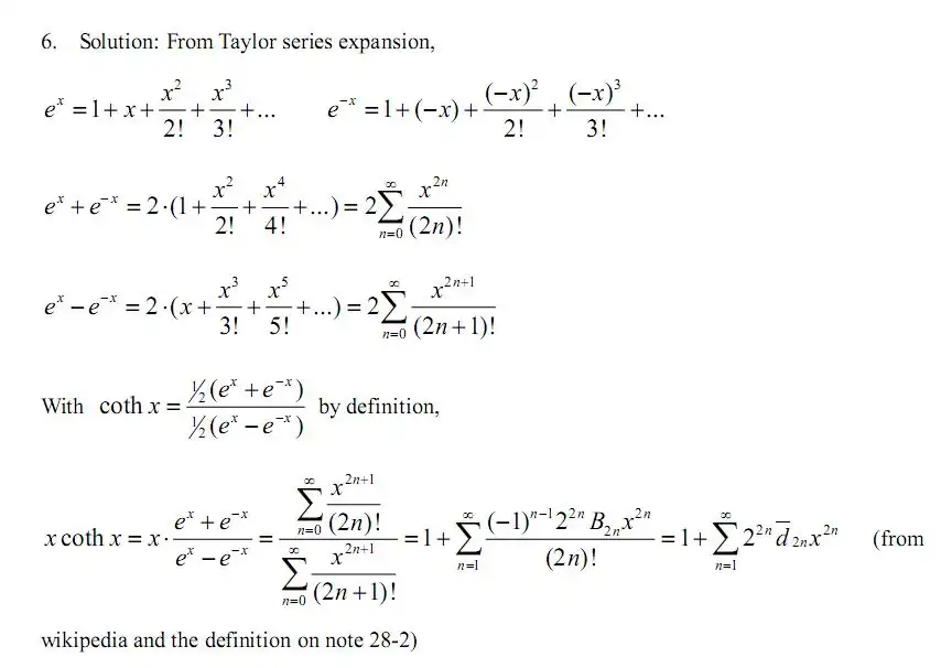
Problem 6: Derivation of terms using Taylor expansion of the hyperbolic function

Statement
P. 28-2 bernoulli nos
Solution

Author
Egm6341.s10.team2.lee 10:12, 26 March 2010 (UTC)
Problem 7: Understanding the derivation of the proof of Trapezoidal Error
Statement
Redo steps in the proof of the Trapezoidal Rule error by trying to cancel terms with odd order derivatives of "g"
Solution
We begin with equation (5) on P. 21-1 which is the result of transformation of variables on equation (1) P. 21-1
(Prob 4 HW4) (P. 21-1)
![{\displaystyle \displaystyle E_{n}^{1}={\frac {h}{2}}\sum _{k=0}^{n-1}[\int _{-1}^{1}g_{k}(t)dt-[g_{k}(-1)+g_{k}({+1})]]}](../../../../I/1e148dfc1c782ebec210d1d746b18f5421d22a25.svg)
From Prob 5 HW4, we can express the above equation as:
(1)
![{\displaystyle \displaystyle E_{n}^{1}={\frac {h}{2}}\sum _{k=0}^{n-1}[\int _{-1}^{+1}(-t)g^{(1)}(t)dt]}](../../../../I/23ba69610a19e3c0b3f1c8ffc15fb07f922d0f58.svg)
Integrating the term withing the square brackets by "Integration by parts" Prob 7 HW4 we can rewrite (1) as follows
(2)
![{\displaystyle \displaystyle E_{n}^{1}={\frac {h}{2}}\sum _{k=0}^{n-1}[[P_{2}(t)g^{(1)}(t)]_{-1}^{+1}-\int _{-1}^{+1}P_{2}(t)g^{(2)}(t)dt]}](../../../../I/71743df11bc628a2c222acf156b3be5c29407da9.svg)
In order to eliminate terms with even powers of we need to remove terms with odd derivatives of .Therefore, the boundary term in eqn (2) above must be set to zero by selection of .


We have from eqns (1 and 2)P. 21-3
(1)p21-3
(2)p21-3


Setting gives and hence we get


(3)
So following this method, the next term to be eliminated will have P4(t)
(4)

Setting and solving we get .Continuing on these lines we get the eqn (2) in the form


(5)
![{\displaystyle \displaystyle E_{n}^{1}={\frac {h}{2}}\sum _{k=0}^{n-1}{[P_{2}g^{(1)}]_{-1}^{+1}-[P_{3}g^{(2)}]_{-1}^{+1}}+[P_{4}g^{(3)}]_{-1}^{+1}-[P_{5}g^{(4)}]_{-1}^{+1}+[P_{6}g^{(5)}]_{-1}^{+1}-[P_{7}g^{(6)}]_{-1}^{+1}-\int _{-1}^{+1}P_{7}g^{(7)}dt}](../../../../I/3968df3b7795984f9a47cafd402118ef6bc0463d.svg)
Dropping all the terms with odd order derivatives of we get

(6)
![{\displaystyle \displaystyle E_{n}^{1}={\frac {h}{2}}\sum _{k=0}^{n-1}{-[P_{3}g^{(2)}]_{-1}^{+1}}+-[P_{5}g^{(4)}]_{-1}^{+1}+-[P_{7}g^{(6)}]_{-1}^{+1}-\int _{-1}^{+1}P_{7}g^{(7)}dt}](../../../../I/5f8fd6e40e5669cd2a71a7589b851751090750ac.svg)
In general on integrating "m" times we get:
(7)
![{\displaystyle \displaystyle E_{n}^{1}={\frac {h}{2}}\sum _{k=0}^{n-1}(\sum _{i=1}^{m}-[P_{(2i+1)}g^{(2i)}]_{-1}^{+1})-\int _{-1}^{+1}P_{(2m+1)}g^{(2m+1)}dt}](../../../../I/ce9ca8e8f3c0dce7b271ea5247ba04ad8b317546.svg)
manipulating the terms yields,
(8)
![{\displaystyle \displaystyle E_{n}^{1}={\frac {h}{2}}\sum _{k=0}^{n-1}[\sum _{i=1}^{m}-[(P_{(2i+1)}(+1)g^{(2i)}(+1))-(P_{(2i+1)}(-1)g^{(2i)}(-1))]-\int _{-1}^{+1}P_{(2m+1)}g^{(2m+1)}dt}](../../../../I/5f77cf155d7f535da2d074188d0bc69bb73430a0.svg)
Transforming g(t) back to f(x) we get [see [prob 6 HW4]
(9)
![{\displaystyle \displaystyle E_{n}^{1}=\sum _{i=1}^{m}({\frac {h}{2}})^{2i+1}\sum _{k=0}^{n-1}[(P_{(2i+1)}(-1)(f^{(2i)}(x_{k}))-(P_{(2i+1)}(+1)f^{(2i)}(x_{k+1}))]-({\frac {h}{2}})^{2m+1}\sum _{k=0}^{n-1}(\int _{x_{k}}^{x_{k+1}}P_{(2m+1)}(x)f^{(2m+1)}(x))dx)}](../../../../I/5b0b831271dea4f20372ca40b42916e529ae7b3b.svg)
Since the polynomial is odd, it can be extracted out to give the eqn in the form
(9)
![{\displaystyle \displaystyle E_{n}^{1}=\sum _{i=1}^{m}({\frac {h}{2}})^{2i+1}P_{(2i+1)}(-1)\left[\sum _{k=0}^{n-1}[(f^{(2i)}(x_{k})+f^{(2i)}(x_{k+1})]\right]-({\frac {h}{2}})^{2m+2}\sum _{k=0}^{n-1}(\int _{x_{k}}^{x_{k+1}}P_{(2m+1)}(x)f^{(2m+1)}(x))dx)}](../../../../I/dbcd6fd85c35cce24a8921f91de7ea47510727e5.svg)
The problem with this formula is evident at first sight, from this expression.The HO derivatives add up in the first term of the expression and since they will not cancel out (9) cannot be reduced to a simpler form. To see the difference in the two approaches more clearly we compare the equations from the two methods. From (1) P. 27-1 we have
(10)
(9)
![{\displaystyle \displaystyle E_{n}^{1}=\sum _{r=1}^{l}h^{2r}d_{2r}[f^{(2r-1)}(b)-f^{(2r-1)}(a)]-{\frac {h^{(2l)}}{2^{(2l)}}}\sum _{k=0}^{n-1}\int _{x_{k}}^{x_{k+1}}P_{2l}(t_{k}(x))f^{(2l)}(x)dx}](../../../../I/c4b3b0d0ff6756bfcea6898c0fc42c20bf5ecafb.svg)
Comparing the eqns 9 and 10 we see that the first term on 9 has a summation of HO derivatives at different points in the square brackets as opposed to 10 which has the difference of the higher order derivative at only the end points. In this lies the difference of the two methods. 10 is general and easier to apply as we need to evaluate the differential of F(x) at only the end points while 9 is computationally cumbersome since it needs the derivative evaluated at all points.
Author
--Egm6341.s10.team2.niki 14:52, 24 March 2010 (UTC)
Problem 8: Calculating the coefficients and the pairs of polynomials using the Recurrence formula


Statement
Use the recurrence formula on P.29-2 to obtain the coefficients and expressions of the pairs of polynomials
Solution
We know the recurrence formulae:
![{\displaystyle P_{2i}(t)=\sum _{j=0}^{i}C_{2j+1}\;{\frac {t^{2(i-j)}}{[2(i-j)]!}}}](../../../../I/5aa872612c317b59de51a7bde57b242e46144356.svg)

![{\displaystyle P_{2i+1}(t)=\sum _{j=0}^{i}C_{2j+1}\;{\frac {t^{2(i-j)+1}}{[2(i-j)+1]!}}+C_{2i+2}}](../../../../I/e6d1d0adfd37ec8b4b0647737e9981db0ed51491.svg)
Since all the polynomials are odd functions and are set to zero at +1 and -1, we have:

![{\displaystyle P_{2i+1}(1)=\sum _{j=0}^{i}C_{2j+1}\;{\frac {1}{[2(i-j)+1]!}}=0}](../../../../I/5151302990007e9dbe0c160155a71947df6baf70.svg)
![{\displaystyle \sum _{j=0}^{1}C_{2j+1}\;{\frac {1}{[2(1-j)+1]!}}=0\Rightarrow {\frac {C_{1}}{3!}}+{\frac {C_{3}}{1!}}=0\;\Rightarrow {\frac {C_{3}}{1!}}=-{\frac {C_{1}}{3!}}=-{\frac {(-1)}{3!}}={\frac {1}{6}}}](../../../../I/a406a7c00866793fa73348cb245c819a6b09363b.svg)
similarly,
![{\displaystyle \sum _{j=0}^{2}C_{2j+1}\;{\frac {1}{[2(2-j)+1]!}}=0\Rightarrow {\frac {C_{1}}{5!}}+{\frac {C_{3}}{3!}}+{\frac {C_{5}}{1!}}=0\;\Rightarrow {\frac {C_{5}}{1!}}=-{\frac {C_{1}}{5!}}-{\frac {C_{3}}{3!}}=-{\frac {(-1)}{5!}}-{\frac {\frac {1}{6}}{3!}}={\frac {-7}{360}}}](../../../../I/780c1310c7b249303f553da2c309d69907d4bed3.svg)
![{\displaystyle \sum _{j=0}^{3}C_{2j+1}\;{\frac {1}{[2(3-j)+1]!}}=0\Rightarrow {\frac {C_{1}}{7!}}+{\frac {C_{3}}{5!}}+{\frac {C_{5}}{3!}}+{\frac {C_{7}}{1!}}=0\;\Rightarrow {\frac {C_{7}}{1!}}=-{\frac {C_{1}}{7!}}-{\frac {C_{3}}{5!}}-{\frac {C_{5}}{3!}}=-{\frac {(-1)}{7!}}-{\frac {\frac {1}{6}}{5!}}-{\frac {\frac {-7}{360}}{3!}}={\frac {31}{15120}}}](../../../../I/fe698ac8c64165e1afac6132325bd496eb8af9a4.svg)
Now evaluating the polynomials using the coefficients:
![{\displaystyle P_{2}(t)=\sum _{j=0}^{1}C_{2j+1}\;{\frac {t^{2(1-j)}}{[2(1-j)]!}}=C_{1}{\frac {t^{2}}{2!}}+C_{3}=-{\frac {t^{2}}{2}}+{\frac {1}{6}}}](../../../../I/4d74f4b28197944d1e57ad24125d6eb3963db681.svg)
![{\displaystyle P_{3}(t)=\sum _{j=0}^{1}C_{2j+1}\;{\frac {t^{[2(1-j)+1]}}{[2(1-j)+1]!}}=C_{1}{\frac {t^{3}}{3!}}+C_{3}{\frac {t^{1}}{1!}}=-{\frac {t^{3}}{6}}+{\frac {t}{6}}}](../../../../I/822f1badca59a32d4aa668be3d55db94aaca8ae9.svg)
Similarly,
![{\displaystyle P_{4}(t)=\sum _{j=0}^{2}C_{2j+1}\;{\frac {t^{2(2-j)}}{[2(2-j)]!}}=C_{1}{\frac {t^{4}}{4!}}+C_{3}{\frac {t^{2}}{2!}}+C_{5}{\frac {t^{0}}{0!}}=-{\frac {t^{4}}{24}}+{\frac {t^{2}}{12}}-{\frac {7}{360}}}](../../../../I/3f086a81f76ab02e978f81966687b568351031f0.svg)
![{\displaystyle P_{5}(t)=\sum _{j=0}^{2}C_{2j+1}\;{\frac {t^{[2(2-j)+1]}}{[2(2-j)+1]!}}=C_{1}{\frac {t^{5}}{5!}}+C_{3}{\frac {t^{3}}{3!}}+C_{5}{\frac {t^{1}}{1!}}=-{\frac {t^{5}}{120}}+{\frac {t^{3}}{36}}-{\frac {7t}{360}}}](../../../../I/70368088a230444539814c0248dc39992251bef6.svg)
![{\displaystyle P_{6}(t)=\sum _{j=0}^{3}C_{2j+1}\;{\frac {t^{2(3-j)}}{[2(3-j)]!}}=C_{1}{\frac {t^{6}}{6!}}+C_{3}{\frac {t^{4}}{4!}}+C_{5}{\frac {t^{2}}{2!}}+C_{7}=-{\frac {t^{6}}{720}}+{\frac {t^{4}}{144}}-{\frac {7t^{2}}{720}}+{\frac {31}{15120}}}](../../../../I/5ff11c9c9537b4e73bef3f93aed0981c5eaa6670.svg)
![{\displaystyle P_{7}(t)=\sum _{j=0}^{3}C_{2j+1}\;{\frac {t^{[2(3-j)+1]}}{[2(3-j)+1]!}}=C_{1}{\frac {t^{7}}{7!}}+C_{3}{\frac {t^{5}}{5!}}+C_{5}{\frac {t^{3}}{3!}}+C_{7}{\frac {t^{1}}{1!}}=-{\frac {t^{7}}{5040}}+{\frac {t^{5}}{720}}-{\frac {7t^{3}}{2160}}+{\frac {31t}{15120}}}](../../../../I/0de3db0b407d2583a46db1bb2508925c0fb0ccf7.svg)
Author
Srikanth Madala (SM)
Problem 9: Understanding the Matlab code on Kessler paper
Statement
To write a explanatory commentary on kessler's Matlab code for the evaluation of polynomials and their coefficients in the Trapezoidal error P. 30-2
Solution
Matlab code
function [c,p]= traperror(n)
%compute the coefficients p_2, p_4, ... , p_{2n} associated with the
%trapezoidal rule error expansion. Also compute c_1, c_3, ...

f=1; g=2; %defining variables 'f,g,cn and cd'
cn=-1; cd=1;

for k=1:n %beginning of 'for' loop with 'n' as the input value of 'traperror' function

f=f.*g.*(g+1); %reassigning the value of f by using element-wise multiplication of matrix f,g

[newcn,newcd]=fracsum(-1*cn,cd.*f); %calling the function 'fracsum' and passing the arguments n=-1*cn and d=cd.*f to the function fracsum(n,d).
%The function fracsum returns the values [nsum,dsum] which are stored in [newcn,newcd]

cn=[cn;newcn]; cd=[cd;newcd]; % the 'cn' (numerator of the coefficient)  and 'cd' (denominator of the coefficient) values are reassigned in
%the execution of the For loop. In each iteration of the for loop, the new values of 'cn' and 'cd' matrices are incremented by one additional
%column element 'newcn' and 'newcd' respectively

f=[f;1]; %the 'f' matrix is incremented by an additional column element=1, in each iteration of the for loop

g=[2+g(1);g]; % the 'g' matrix is incremented by an additional column element=even number, in each iteration of the for loop

[newpn,newpd]=fracsum((g-1).*cn,f.*cd);%calling the function 'fracsum' and passing the arguments n=(g-1).*cn and d=f.*cd to the function fracsum(n,d).
%The function fracsum returns the values [nsum,dsum] which are stored in [newpn,newpd]

pn(k,1)=newpn; % each numerator element of the polynomial function is stored in a column matrix with 'k' rows

pd(k,1)=newpd;  % each denominator element of the polynomial function is stored in a column matrix with 'k' rows

end % end of for loop to check and see if k=n?

c=int64([cn cd]); % converts the numerator and denominator of the coefficient to signed 64-bit integers

p=int64([pn pd]); % converts the numerator and denominator of the polynomial function to signed 64-bit integers

%%%%%%%%%%%%%%%%%%%%%%%%%%%%%%%%%%%%%%%%%%%%%%%%%%%%%%%%%%%%%%%%%%%%%%%%%%%%%%%%%%%%%%%%%%%%%%%%%%%%%%%%%%%%%%%%%%%%%%%%%%%%%%%%%%%%%%%%%%%%%%

function [nsum,dsum]= fracsum(n,d) %the arguments 'n' and 'd' are passed to this function and the output of this function are 'nsum' and 'dsum'

div=gcd(round(n),round(d)); %'round' is a matlab function to rounding off the fraction to the nearest integer and 'gcd' is a matlab function that
%returns the greatest common divisor of round(n) and round(d). This value of gcd is stored in a variable 'div'

n=round(n./div); % 'n' matrix is reassigned by carrying out element wise division with 'div' and then rounding off

d=round(d./div); % 'd' matrix is reassigned by carrying out element wise division with 'div' and then rounding off

dsum=1; % a new variable 'dsum' is initially assigned a value of 1

for k=1:length(d) % a new 'for' loop is started

dsum=lcm(dsum,d(k)); %'lcm' is a matlab function that returns the lowest common multiple of the values in the parentheses and in this case dsum and d(k)

end % end of for loop to check and see if k=length(d)?

nsum=dsum*sum(n./d); %'nsum' variable is defined by carrying out the arithemetic operation between 'dsum' and sum(n./d)

div=gcd(round(nsum),round(dsum)); %'div' is reassigned a different value which is the GCD of rounded values of 'nsum' and 'dsum'

nsum=nsum/div; %'nsum' is redefined
Author
Srikanth Madala (SM)
Problem 10: Calculating the Circumference of an ellipse
Statement
An Ellipse as given:

where:


Calculate the Circumference of the elipse as follows:
Method 1:
![{\displaystyle C=\int _{0}^{2\pi }\left[r^{2}+({\frac {dr}{d\theta }})^{2}\right]^{\frac {1}{2}}}](../../../../I/471e6e3ba33905143c06ac39ffedc7fa2d1f31af.svg)
Method 2:

![{\displaystyle E(e^{2})=\int _{0}^{\frac {\pi }{2}}\left[1-e^{2}\sin(\theta )\right]^{\frac {1}{2}}d\theta }](../../../../I/eb9cd39748e94809c716210bea08e2fce5aa0e19.svg)
Method 1
The Circumference will be calculated by using the following:
And then integrated numerically using 3 methods:
- Composite Trapezoidal
- Clencurt
- Romberg Table
The approximation for the exact integral was calculated using the "quad" Matlab command. It was approximated to be 6.176517851674653
Composite Trapezoidal
Composite Trapezoidal Rule | ||
| n | Value | Error |
| 2 | 6.283099768855828 | 0.106581917181175 |
| 4 | 6.169238034994176 | 0.007279816680477 |
| 8 | 6.176493841410109 | 2.401026454457167e-005 |
| 16 | 6.176517900218237 | 4.854358426342742e-008 |
Matlab code for composite Trapezoidal calculation
%Calculates the Integral using the Composite Trapezoidal Rule
function [I,E]=circompos(a,b,n)

h=(b-a)/n;
pi2=2*pi();
i=0;
Itot=0;
It=0;
It2=0;
%Function elarc calculates the value of the function of the integral as seen in the code below
while i<=n
    if i==0
        Itot1=(1/2)*elarc(a);
    else if i<n
            u=h*i;
            It(i)= elarc(u);
        else
            It2=(1/2)*elarc(b);
        end
    end
Itot=Itot1+sum(It)+It2;
i=i+1;
end

I=Itot*(h);

%Error Calculation compared to built in 'quad' matlab command
Ir=quad(@elarc,0,pi2);
E=Ir-I;
Matlab code for calculation of the integrand
function arc = elarc(t)

%Finding the Circumference of an ellipse

%C=integral(dl) from 0 to 2PI

e=sin(pi()/12);
e2=e^2;
r=(1-.0670)./(1-e.*cos(t));
dr2=(118270190867084615574681258512889*sin(t).^2)./(2028240960365167042394725128601600*((291404338770025.*cos(t))./1125899906842624 - 1).^4);

%Integrand:

arc=(r.^2 + (dr2) ).^(.5);
Clencurt
Clencurt Function | ||
| Value | Error | |
| 6.176517900218237 | 4.854358426342742e-008 | |
Matlab code
   [xx,ww] = clencurt(n);                               %Calls the clencurt function
    xx=pi+xx.*pi;
    ww=ww.*pi;
    F=elarc(xx);  %Evaluation of the function
    I_cl=ww*F
    I=6.176517851674653;
    E=abs(I_cl-I)

function arc = elarc(t)

%Finding the Circumference of an ellipse

%C=integral(dl) from 0 to 2PI

e=sin(pi()/12);
e2=e^2;
r=(1-.0670)./(1-e.*cos(t));
dr2=(118270190867084615574681258512889*sin(t).^2)./(2028240960365167042394725128601600*((291404338770025.*cos(t))./1125899906842624 - 1).^4);

%Integrand:

arc=(r.^2 + (dr2) ).^(.5);
Romberg Table
Romberg Table for n=16
  6.176517900218236   6.176517900385847   6.176517900341150   6.176517900343991   6.176517900343945   6.176517900343941
  6.176517900343945   6.176517900343943   6.176517900343947   6.176517900343945   6.176517900343941                   0
  6.176517900343944   6.176517900343946   6.176517900343945   6.176517900343941                   0                   0
  6.176517900343946   6.176517900343946   6.176517900343941                   0                   0                   0
  6.176517900343946   6.176517900343942                   0                   0                   0                   0
  6.176517900343943                   0                   0                   0                   0                   0
Error of Romberg Table
- 1.0e-007 *
  -0.485435833752490  -0.487111941893659  -0.486664966103945
  -0.486692917078813  -0.486692899315244  -0.486692934842381
  -0.486692908197028  -0.486692925960597  -0.486692917078813
  -0.486692925960597  -0.486692925960597  -0.486692881551676
  -0.486692925960597  -0.486692890433460                   0
  -0.486692899315244                   0                   0
Columns 4 through 6
  -0.486693378931591  -0.486692917078813  -0.486692881551676
  -0.486692917078813  -0.486692881551676                   0
  -0.486692881551676                   0                   0
                   0                   0                   0
                   0                   0                   0
                   0                   0                   0
Romberg Table Results | ||
| Value | Error | |
| 6.176517900343941 | 4.86692881551676e-008 | |
Matlab code
%The Function outputs the romberg table and a table with the error,  the
%inputs are a=low boundary b=high boundary n=initial number of integration
%points for the romberg table
function [table,etable] = elarcromb(a,b,n)
tic
table=zeros(6,6);

%Generate 1st column of Romberg Table using built in composite trapezoidal
%function.  Notice it calls the function 'Valus' which obtains the values
%for the function.  The function is also corrected at initial point 0
for j=1:6
    r=n;
    x=linspace(a,b,r+1);
    FX=elarc(x);
    %FX(1)=1;  %because of 0 start point
    table(j,1)=trapz(x,FX);
    n=2*r;
end

%Generate 2nd column of Romberg Table
for j=1:5
    table(j,2)= ([(2^2)*table(j+1,1)] - [table(j,1)])/(2^2 - 1);
end

%Generate 3rd column of Romberg Table
for j=1:4
    table(j,3) = ([(2^(2*2))*table(j+1,2)] - table(j,2))/(2^(2*2)-1);
end

%Generate 4th column of Romberg Table
for j=1:3
    table(j,4) = ([(2^(2*3))*table(j+1,3)] - table(j,3))/(2^(2*3)-1);
end

%Generate 5th Column of Romberg Table
for j=1:2
    table(j,5) = ([(2^(2*4))*table(j+1,4)] - table(j,4))/(2^(2*4)-1);
end

%Generate 6th column of Romberg Table
table(1,6) = ([(2^(2*5))*table(2,5)] - table(1,5))/(2^(2*5)-1);

%Table of errors for the Romberg Table
etable=zeros(6,6);
pi2=2*pi();
I=quad(@elarc,0,pi2);  %Value found using Quad function of Matlab

%1st column
for i=1:6
    etable(i,1)= I - (table(i,1));
end

%2nd column
for i=1:5
    etable(i,2)= I - (table(i,2));
end

%3rd column
for i=1:4
    etable(i,3)= I - (table(i,3));
end

%4th Column
for i=1:3
    etable(i,4)= I - (table(i,4));
end

%5th column
for i=1:2
    etable(i,5)= I - (table(i,5));
end

%6th Column
etable(1,6) = I - (table(1,6));

toc
Method 2

The integral is calculated using 3 methods:
- Composite Trapezoidal
- "Clencurt" Matlab Command
- Romberg Table
It will then by used to find the circumference as previously stated.
Composite Trapezoidal
Composite Trapezoidal Rule | ||
| n | Value | Error |
| 2 | 1.538588738571503 | 0.001739607794329 |
| 4 | 1.537280664642864 | 4.315338656908363e-004 |
| 8 | 1.536956805756325 | 1.076749791522058e-004 |
| 16 | 1.536855855380622 | 6.724603448970967e-006 |

Romberg Table
  1.536876035753892   1.536849128589532   1.536849129666574   1.536849129666558   1.536849129666558   1.536849129666558
  1.536855855380622   1.536849129599258   1.536849129666558   1.536849129666558   1.536849129666558                   0
  1.536850811044599   1.536849129662352   1.536849129666558   1.536849129666558                   0                   0
  1.536849550007914   1.536849129666295   1.536849129666558                   0                   0                   0
  1.536849234751700   1.536849129666542                   0                   0                   0                   0
  1.536849155937831                   0                   0                   0                   0                   0


Both Methods yield similar but not equal results. Also it is noted that the error associated with method 1 is less than that of method 2
Author
--Egm6341.s10.Team2.GV 22:07, 25 March 2010 (UTC)
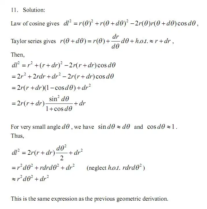
Problem 11: Derivation of infinitesimal arc length using the Law of cosine
Statement
Derive the infinitesimal arc length using the Law of cosine
Solution
Author
Egm6341.s10.team2.lee 08:57, 24 March 2010 (UTC)
Contributing Authors
Signatures
Solved problems 4 and 9. Proofread 5,10--Srikanth Madala (SM)
Solved problem 2 and 7. Proofread 1,3,8,10--Egm6341.s10.team2.niki| Niki Nachappa (NN) 17:17, 24 March 2010 (UTC)
Proofread problems 3, 8, 11--Egm6341.s10.team2.patodon 20:57, 24 March 2010 (UTC)
Solved problems 5 and 10. Proofread 1, 4, 11 --Egm6341.s10.Team2.GV 22:14, 25 March 2010 (UTC)
Solved problems 1,6, 11. Proofread 2, 7, 9 --Egm6341.s10.team2.lee 16:28, 26 March 2010 (UTC)
Solution Assignments and Reviewers
Problem Assignments | ||
| Problem # | Solution | Reviewed |
| Problem 1 | JP | NN,GV |
| Problem 2 | NN | PO,JP |
| Problem 3 | PO | SM,NN |
| Problem 4 | SM | GV,PO |
| Problem 5 | GV | JP,SM |
| Problem 6 | JP | PO,GV |
| Problem 7 | NN | SM,JP |
| Problem 8 | PO | GV,NN |
| Problem 9 | SM | JP,PO |
| Problem 10 | GV | NN,SM |
| Problem 11 | JP | PO,GV |