University of Florida/Egm6341/s10.Team2/HW7
problem 1: Stable Growth for Verhulst Equation
Statement
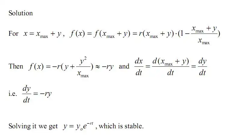
Pg.38-4 Show the case of stable growth for Verhulst equation
Solution
Author
Egm6341.s10.team2.lee 20:56, 23 April 2010 (UTC)
problem 2: Solution of the Logistic equation
Statement
Solution
We have Verhulst model or the Logistic equation as P.38-3

Separating variables and integrating we have

which can be written as

We get


Rearranging we have

Author
--Egm6341.s10.team2.niki 12:31, 23 April 2010 (UTC)
problem 3: Hermite-Simpson Algorithm to solve for the non-linear first order differential equation i.e. Verhulst population growth model on Pg.38-3
Statement
Use the Hermit-Simpson Algorithm to integrate the Verhulst population growth model on Pg.38-3:

Consider the following: and
Case 1:
Case 2:
![{\displaystyle x_{max}=10\;\;r=1.2\;\;t\in \left[0,10\right]}](../../../../I/aca5030c379bec9c6fbe3f8dc89eb31b755d5d8a.svg)


And also plot the two cases using matlab.
Solution
Matlab code
%Matlab code to integrate the the Verhulst population growth model
clear;
clc;
xmax=10;
r=1.2;
t=0:0.1:10;
h=0.1; %time step size
syms x;
syms x11;
f=r*x*(1-(x/xmax));
%case 1: when x0=2
for i=1:1:100
    x1(1)=2;
    f1=subs(f,x,x1(i));
    f11=subs(f,x,x11);
    x1half=((1/2)*(x1+x11))+((h/8)*(f1-f11));
    f1half=subs(f,x,x1half);
    F=x1(i)-x11+(h/6)*(f1+f11+(4*f1half));
    guessx11(i)=x1(i);
    dummy=1;
    while dummy==1
    newx11(i)=guessx11(i)-((1/(subs(diff(F(i)),x11,guessx11(i))))*(subs(F(i),x11,guessx11(i))));
    if double(abs(newx11(i)-guessx11(i)))<=10^(-6)
       x1(i+1)=newx11(i);
       dummy=0;
        break;
    else
        guessx11(i)=newx11(i);
        dummy=1;
    end
    end
end
plot(t,x1);
THE PLOT SHOWING THE POPULATION CHANGE W.R.T TIME, HERE VERHULST MODEL IS USED TO COMPUTE THE POPULATION WHERE XO=INITIAL POPULATION=2

THE PLOT SHOWING THE POPULATION CHANGE W.R.T TIME, HERE VERHULST MODEL IS USED TO COMPUTE THE POPULATION WHERE XO=INITIAL POPULATION=7

Author
Solved by--Srikanth Madala (SM)
Problem4: Creating graphs, showing the bifurcation diagram for the logistic map and its sensitivity to initial conditions
Statement
Produce the diagrams showing the bifurcation diagram for the logistic map and its sensitivity to initial conditions, as shown on figures 15.6 and 15.7, of the book "Differential Equations: Linear,Nonlinear,Ordinary,Partial" by King,Billingham and Otto (Pg.455-456).
Solution
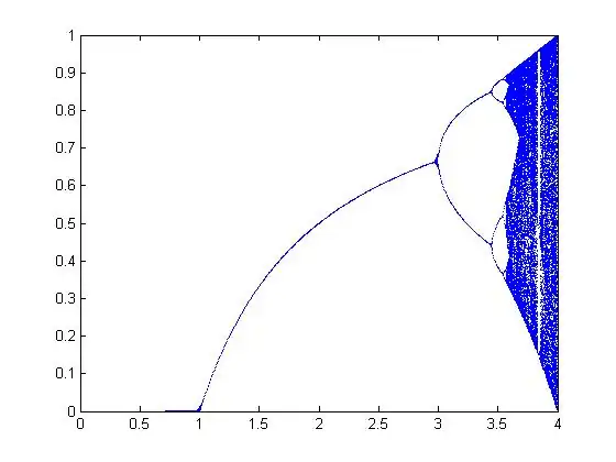
Creating Figure 15.6:Bifurcation Diagram
Logistic Map:

The Bifurcation Diagram shows the period doubling process of the logistic map. As the constant r increases the period is doubled to 2 periods and then stability is lost which then leads to a doubling of period to 4 and so on.
The plot is as follows:
Matlab Code
Matlab code used to create the graph as outlined in Pg. 455 of King et. al
for r= 0:0.005:4
    x=rand(1);
    for j = 1:100
        x=r*x*(1-x);
    end
    xout=[];
    for j=1:400
        x=r*x*(1-x); xout=[xout x];
    end
    plot (r*ones(size(xout)),xout,'.','MarkerSize',3)
    axis([0 4 0 1]), hold on, pause(0.01)
end
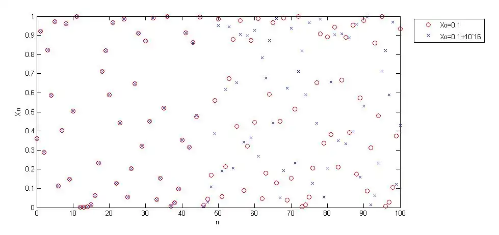
Creating Figure 15.7: Sensitivity to Initial Conditions
The Following Plot explores the big effect of a small change in the initial conditions. One can note the changes as 'n' becomes larger than 50. The graph was produced for the following Conditions:

The Following Equation was used to produce the iterations for the graph:
Matlab Code
Matlab Code used to produce the aforementioned plot.
function [xn1 xn2]=fig157

r=4;

format long

x01=.1;
x02=0.1+(10^-16);

for j=0:100
k=j+1;
x1=r*x01.*(1-x01);
x2=r*x02.*(1-x02);

xn1(k,1)=x1;
xn2(k,1)=x2;

x01=x1;
x02=x2;

end

n=0:100;
plot(n,xn1,'o')
hold on
plot(n,xn2,'x')
Author
--Egm6341.s10.Team2.GV 16:28, 23 April 2010 (UTC)
problem 5: Variation of the plot with the increase in the time step size
Statement
Solution
Matlab code
clear;
clc;
xmax=10;
r=1.2;
t=0:0.1:10;
h=0.1; %time step size
syms x;
syms x11;
f=r*x*(1-(x/xmax));
%case 1: when x0=2
for k=1:1:5
    h=2*h;
for i=1:1:100
    x1(1)=2;
    f1=subs(f,x,x1(i));
    f11=subs(f,x,x11);
    x1half=((1/2)*(x1+x11))+((h/8)*(f1-f11));
    f1half=subs(f,x,x1half);
    F=x1(i)-x11+(h/6)*(f1+f11+(4*f1half));
    guessx11(i)=x1(i);
    dummy=1;
    while dummy==1
    newx11(i)=guessx11(i)-((1/(subs(diff(F(i)),x11,guessx11(i))))*(subs(F(i),x11,guessx11(i))));
    if double(abs(newx11(i)-guessx11(i)))<=10^(-6)
       x1(i+1)=newx11(i);
       dummy=0;
        break;
    else
        guessx11(i)=newx11(i);
        dummy=1;
    end
    end
end
plot(t,x1);
hold on
end
THE PLOT SHOWING THE POPULATION CHANGE W.R.T TIME, HERE VERHULST MODEL IS USED TO COMPUTE THE POPULATION WHERE XO=INITIAL POPULATION=2
color scheme in the plot below | ||
| Color | h-value | |
| Red | h=0.2 | |
| Blue | h=0.4 | |
| Green | h=0.8 | |
| Magenta | h=1.6 | |
| Brown | h=3.2 | |

Author
Solved by--Srikanth Madala (SM)
Problem6: Solving Ordinary Differential Equations using Euler Implicit Methods
Statement
Solve the following Group of ODE's as they relate to the problem mentioned in the lecture pages mentioned above. The problem is of the motion of an airplane through different maneuvers.
for a vector with the following parameters:
![{\displaystyle z=[x,y,V,\gamma ]}](../../../../I/13f30200f2bbccf3637f43ee4572c76cdfaf9850.svg)
![{\displaystyle {\dot {z}}=[{\dot {x}},{\dot {y}},{\dot {V}},{\dot {gamma}}]}](../../../../I/528141f5dbd0754cadeaf3acdd0e477f2cb26716.svg)


Initial Conditions are as follows:


The Physical Modeling Parameters to be used are


The Inputs are defined as follows:
Input T:
for
for
for


Input :

for
for as it varies linearly
for as it varies linearly
for as it varies linearly


Solution
Defining the Inputs
The first part of the solution is to create a function that will calculate the thrust and angle of a attack at a particular time. The following Matlab Codes were used:
Thrust:
% Function that calculates the thrust for any given time, t
function T = thrust(t)

%for t=0:40
 %   k=t+1;
if (t >= 0) & (t < 27),
   T = 6000;
elseif (t >= 27) & (t < 33),
   T = 1000;
else
   T = 6000;
end;
%end
Angle of Attack:
% Function calculates the angle of attack from 0-40secs
function alpha = angleatak(t)

%for t=0:40
 %   k=t+1;
if (t >= 0) & (t < 21),
   alpha = 0.03;
elseif (t >= 21) & (t < 27),
   alpha = ((0.13-0.09)/(27-21))*(t-21) + 0.09;
elseif (t >= 27) & (t < 33),
   alpha = ((-0.2 + 0.13)/(33-27))*(t-27) - 0.13;
else
   alpha = ((-0.13 +0.2)/(40-33))*(t-33) - 0.2;
end;
%end
Technique used to solve the problem
The overall goal is to find a solution for each of the states being considered (x,y,V,gamma).
From P 36.3, of the lectures, the following was established using the Hermite-Simpson Algorithm:
![{\displaystyle Z_{i+1}=z_{i}+{\frac {h/2}{3}}\left[f_{i}+4f(g(z_{i},z_{i+1}))+f(z_{i+1})\right]\qquad \qquad EQUATION1}](../../../../I/0092f4fc1aecb995c212adbc0d743a668ec510fd.svg)
The Following is recognized and derived as:
![{\displaystyle g(z_{i},z_{i+1})={\frac {1}{2}}(z_{i}+z_{i+1})+{\frac {h}{8}}\left[(f(z_{i})-f(z_{i+1})\right]\qquad \qquad EQUATION2}](../../../../I/9a7c13918fc1f7a5e6212cccc8c8f5cc189f1195.svg)
It is now necessary to define the following using the previously mentioned Eq. 1:
![{\displaystyle F(Z_{i+1})=0=Z_{i+1}-z_{i}-{\frac {h/2}{3}}\left[f_{i}+4f(g(z_{i},z_{i+1}))+f(z_{i+1})\right]\qquad \qquad EQUATION3}](../../../../I/9e8a675adc1bb1e676c5d5561a2450af1384b038.svg)
The next step is to apply the Newton Raphson Method to solve the function

A Matlab Algorithm is used to apply the Newton Raphson Method as follows:
Newton Raphson Method
Function for obtaining

function f = fcalc(t,z)

% z(1) = x : horizontal position
% z(2) = y : vertical position(height)
% z(3) = v : velocity
% z(4) = gamma : angle to new x-axis

% Set parameters
m = 1005; % kg
g = 9.81; % m/s^2
Sr = 0.3376; % m^2
A1 = -1.9431;
A2 = -0.1499;
A3 = 0.2359;
B1 = 21.9;
B2 = 0;
C1 = 3.312e-9; % kg/m^5
C2 = -1.142e-4; % kg/m^4
C3 = 1.224; % kg/m^3

alpha = angleatak(t); % Call alpha
T = thrust(t); % Call thrust

Cd = A1.*alpha.^2 + A2.*alpha + A3;
Cl = B1.*alpha + B2;
rho = C1*z(4)^2 +C2*z(4) + C3; % density

D = 0.5*Cd*rho*z(3)^2*Sr; % Calculate D
L = 0.5*Cl*rho*z(3)^2*Sr; % Calculate L

f = zeros(4,1);
f(1) = z(2)*cos(z(4));
f(2) = z(2)*sin(z(4));
f(3) = (T-D)*cos(alpha)/m - L*sin(alpha)/m -g*sin(z(4));
f(4) = (T-D)*sin(alpha)/(m*z(3)) + L*cos(alpha)/(m*z(3))-(g*cos(z(4)))/z(3);
Function for obtaining

function df = dfcalc(t,z)

% z(1) = x : horizontal position
% z(2) = y : vertical position(height)
% z(3) = v : velocity
% z(4) = gamma : angle to new x-axis

% Set parameters
m = 1005; % kg
g = 9.81; % m/s^2
Sr = 0.3376; % m^2
A1 = -1.9431;
A2 = -0.1499;
A3 = 0.2359;
B1 = 21.9;
B2 = 0;
C1 = 3.312e-9; % kg/m^5
C2 = -1.142e-4; % kg/m^4
C3 = 1.224; % kg/m^3

alpha = angleatak(t); % Call alpha
T = thrust(t); % Call thrust

Cd = A1.*alpha.^2 + A2.*alpha + A3;
Cl = B1.*alpha + B2;
rho = C1*z(4)^2 +C2*z(4) + C3; % density

D = 0.5*Cd*rho*z(3)^2*Sr; % Calculate D
L = 0.5*Cl*rho*z(3)^2*Sr; % Calculate L

%Caculates DF
df=zeros(4,4);
df(1,1) = 0; %
df(1,2) = 0; %
df(1,3) = cos(z(4));
df(1,4) = -z(3)*sin(z(4));

df(2,1) = 0;
df(2,2) = 0;
df(2,3) = sin(z(4));
df(2,4) = z(2)*cos(z(1));

df(3,1) = 0;
df(3,2) = -Cd*(2*C1*z(4)+C2)*z(2)^2*Sr*cos(alpha)/(2*m) - Cl*(2*C1*z(4)+C2)*z(2)^2*Sr*sin(alpha)/(2*m);
df(3,3) = -Cd*rho*z(3)*Sr*cos(alpha)/m - Cl*rho*z(3)*Sr*sin(alpha)/m;
df(3,4) = -g*cos(z(4));

df(4,1) = 0;
df(4,2) = -Cd*(2*C1*z(2)+C2)*z(3)*Sr*sin(alpha)/(2*m) + Cl*(2*C1*z(2)+C2)*z(3)*Sr*cos(alpha)/(2*m);
df(4,3) = -T*sin(alpha)/(m*z(3)^2) - Cd*rho*Sr*sin(alpha)/(2*m) + Cl*rho*Sr*cos(alpha)/(2*m) + g*cos(z(4))/z(3)^2;
df(4,4) = g*sin(z(4))/z(3);
Function for using the Newton Raphson Operations until an error threshold is reached
This Matlab code was developed using the published code of Team 3 as part of their HW 7 Report( HW 7: Team 3)
% This function returns the solution of EOMs given
% in Subchan and Zbikowski, Optim. Control Appl. Meth. 2007; 28:311-353.
% This function uses Hermite-Simpson (HS) algorithm and Newton-Raphson (NR) method.
% Note:
% z_out(time,1) = gamma : angle b/w aircraft body and x-axis for a given time
% z_out(time,2) = v : aircraft velocity for a given time
% z_out(time,3) = x : x-coordinate of aircraft for a given time
% z_out(time,4) = y : y-coordinate of aircraft for a given time
% t_out = times corresponding to nodes
function [t,z] = NRplane

i = 0;

% This "while" loop is for increasing # of nodes to achieve the given tolerance
while (true),
   i = i + 1; % # of iterations
   n = 2^(i-1); % # of subinterval

   tinit = 0.0; % initial time (sec)
   tfinal = 40.0; % final time (sec)

   %initial conditions
   z0 = zeros(4,1);
   z0(1) = 0;
   z0(2) = 30;
   z0(3) = 272;
   z0(4) = 0;
   f0 = fcalc(tinit,z0); % Call f(z) for t = 0

   h = (tfinal - tinit)/n; % time step

   z_out = zeros(n+1,4); % output solution
   t_out = zeros(n+1,1); % output time evolution

   % assign the initial conditions to the solution for t = 0
   z_out(1,1) = z0(1); z_out(1,2) = z0(2);
   z_out(1,3) = z0(3); z_out(1,4) = z0(4);
   t_out(1) = tinit;

   % We need the values of previous time step in HS algorithm
   zj_p = zeros(4,1); % a column vector
   zj_p(1) = z0(1); zj_p(2) = z0(2);
   zj_p(3) = z0(3); zj_p(4) = z0(4);
   tj_p = tinit;

   % This "for" loop is for time evolution.
   % "j = 1" corresponds to t = tinit and "j = n+1" corresponds to t = tfinal
   for j = 2:n+1,
       tj = tinit + (j-1)*h; % current time
       zj = zj_p; % initial guess for NR method
       k = 0;
       % This "while" loop is for NR method.
       while (true),
          k = k + 1;
          fb_p = fcalc(tj_p,zj_p); % Call f(z) for t = t(j)
          fb = fcalc(tj,zj); % Call f(z) for t = t(j+1)

          tj_md = 0.5*(tj_p + tj); % t = t(i+1/2)
          g = 0.5*(zj_p + zj) + (h/8)*(fb_p - fb); % Obtain z for t = t(j+1/2)
          fb_md = fcalc(tj_md,g); % Call f(z) for t = t(j+1/2)

          % Calculate F(z) for t = t(j+1)
          ff = zj - zj_p - (h/6)*(fb_p + 4.0*fb_md + fb);

          dfb = dfcalc(tj,zj); % Call df/dz for t = t(j+1)
          dg = 0.5*eye(4,4) - (h/8)*dfb; % Calculate dg/dz for t = t(j+1)
          dfbdg = dfcalc(tj_md,g); % Call df/dz for t = t(j+1/2)

          % Calculate dF/dz for t = t(j+1)
          dff = eye(4,4) - (h/6)*(4.0*dfbdg*dg + dfb);
          inv_dff = inv(dff); % obtain inverse of dF/dz
          zj_f = zj - inv_dff*ff; % Calculte new solution z for t = t(j+1)

          % Check tolerance
          if (norm(abs(zj_f-zj),inf) < 1.e-6),
             break;
          end;

          % Redo interation if the error is still larger than tolerance
          zj = zj_f;
       end;

       % Assign the satisfied solution to the output matrices
       t_out(j) = tj;
       z_out(j,1) = zj_f(1); z_out(j,2) = zj_f(2);
       z_out(j,3) = zj_f(3); z_out(j,4) = zj_f(4);

       % Current values become previous values for the next time step
       tj_p = tj;
       zj_p = zj_f;
   end;

   % check tolerance
   if (i ~= 1) & (norm(abs(zj_f - zj_fp),inf) < 1.e-2),
      break;
   end;

   zj_fp = zj_f;
end;
Results of Methods Used and comparison to ODE45
Plot of Horizontal Position Vs. Time
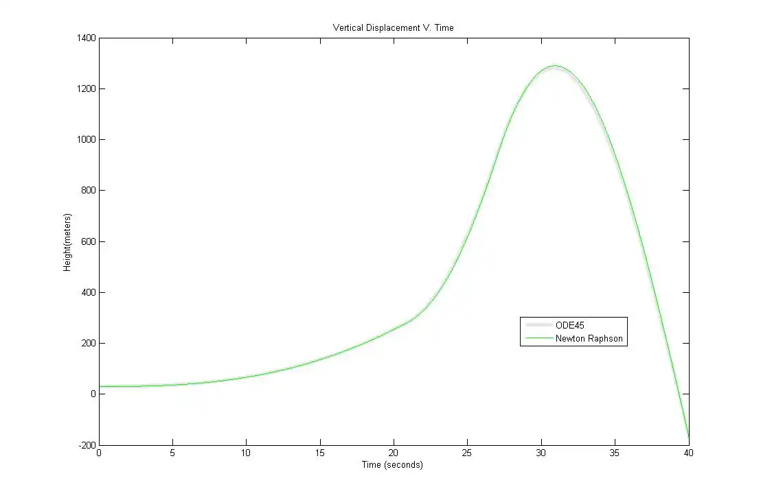
Plot of Vertical Position(Height) Vs. Time
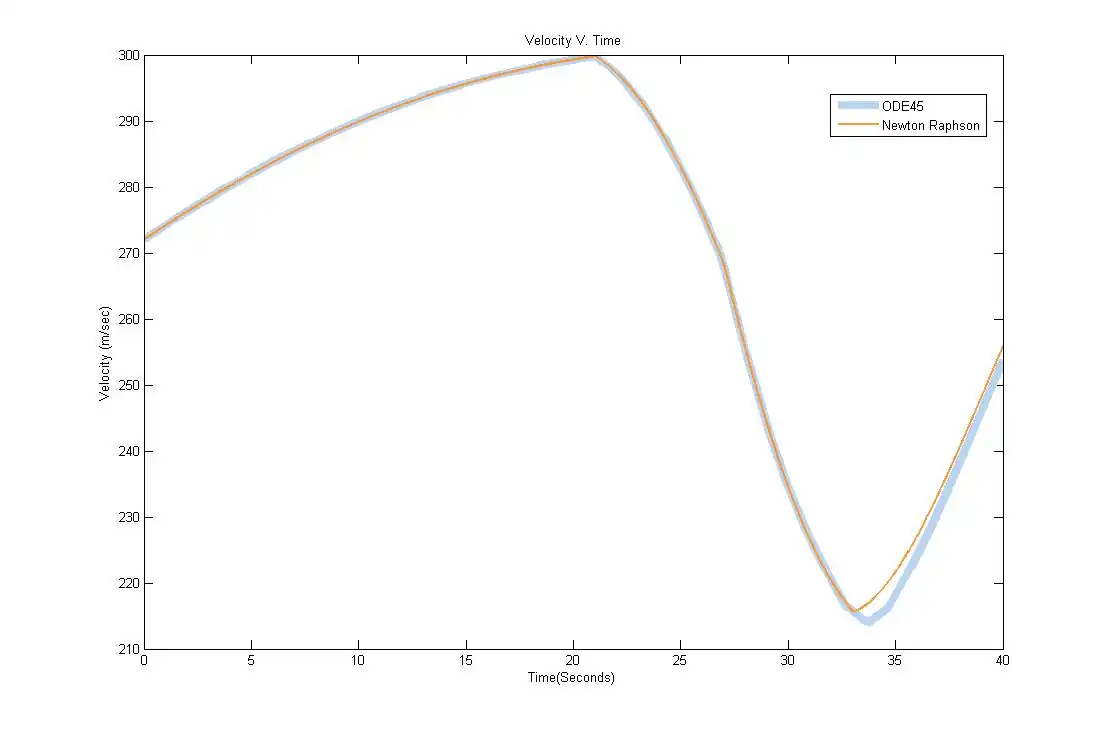
Plot of Velocity Vs. Time
Plot of Gamma Vs. Time
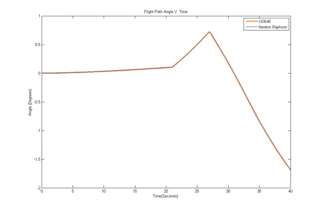
From each of these plots it can be concluded that the combination of the Hermite Simpson Algorith and the Newton Raphson Method is an effective way to solve the set of ordinary differential equations without much error, as compared to ODE45 solver of Matlab. The downside to this method is that it takes a high amount of computational resources and time.
Author
--Egm6341.s10.Team2.GV 23:41, 27 April 2010 (UTC)
problem7 :Integration of Logistic equation by
Statement
Integrate the Logistic equation using the inconsistent Trapezoidal-Simpson approximation

Solution
The Matlab code is a slight alteration of the code used to integrate above.
  %Matlab code to integrate the the Verhulst population growth model
  clear;
  clc;
  xmax=10;
  r=1.2;
  t=0:0.1:10;
  h=0.1; %time step size
  syms x;
  syms x11;
  f=r*x*(1-(x/xmax));
  %case 1: when x0=2
  for i=1:1:100
   x1(1)=2;
   f1=subs(f,x,x1(i));
   f11=subs(f,x,x11);
   x1half=((1/2)*(x1+x11))%Trapezoidal_simpson approxiamtion;
   f1half=subs(f,x,x1half);
   F=x1(i)-x11+(h/6)*(f1+f11+(4*f1half));
   guessx11(i)=x1(i);
   dummy=1;
   while dummy==1
   newx11(i)=guessx11(i)-((1/(subs(diff(F(i)),x11,guessx11(i))))*(subs(F(i),x11,guessx11(i))));
   if double(abs(newx11(i)-guessx11(i)))<=10^(-6)
      x1(i+1)=newx11(i);
      dummy=0;
       break;
   else
       guessx11(i)=newx11(i);
       dummy=1;
   end
   end
  end
  plot(t,x1);
for

for

Author
--Egm6341.s10.team2.niki 20:33, 28 April 2010 (UTC)
problem8
Statement
Solution
Author
Problem9: Eliminating t from the Parameterization of an ellipse
Statement
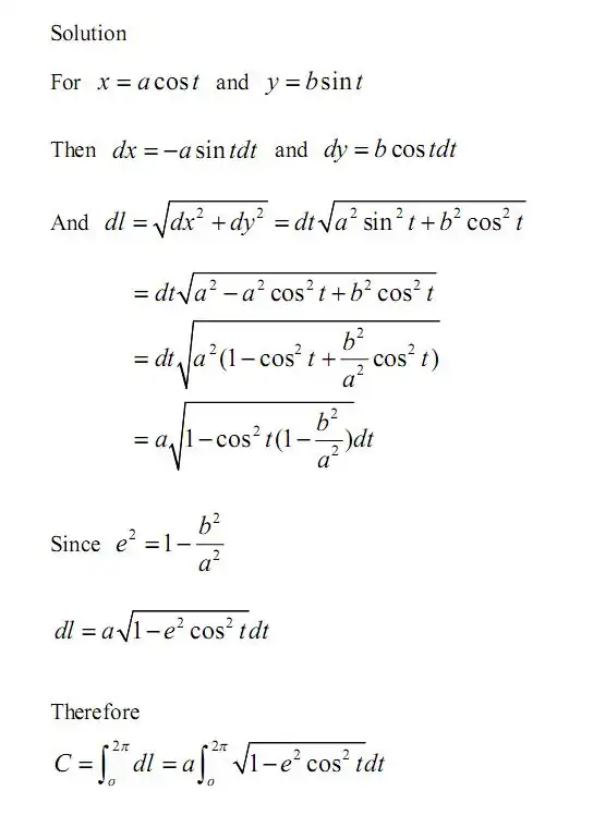
Given the parameterization for an ellipse as follows for the x and y coordinates, Eliminate 't' as a parameter.

Solution


At this point t can be eliminated as a parameter.

Author
--Egm6341.s10.Team2.GV 17:51, 23 April 2010 (UTC)
problem10
Statement
Solution
Author
problem11: To show the integral for elliptical circumference
Statement
Pg.42-2 To show the integral for elliptical circumference
Solution
Author
Egm6341.s10.team2.lee 20:58, 23 April 2010 (UTC)
problem12
Statement
Solution
Author
problem 13: Change of Variable
Statement
To show that

Solution
We have the integral as
.

Using the transformation we have


and using the inverse transformation the limits can be written
![{\displaystyle \displaystyle {[-1,1]}}](../../../../I/619a7d2faa224e30a65b1d05174cd0449d2b9062.svg)
![{\displaystyle \displaystyle {[\pi ,0]}}](../../../../I/033de82ca546a96544218ba1d7e91657d48a6ffd.svg)
thus we have

Author
--Egm6341.s10.team2.niki 18:47, 23 April 2010 (UTC)
problem 14: Constants of the Cosine Series
Statement
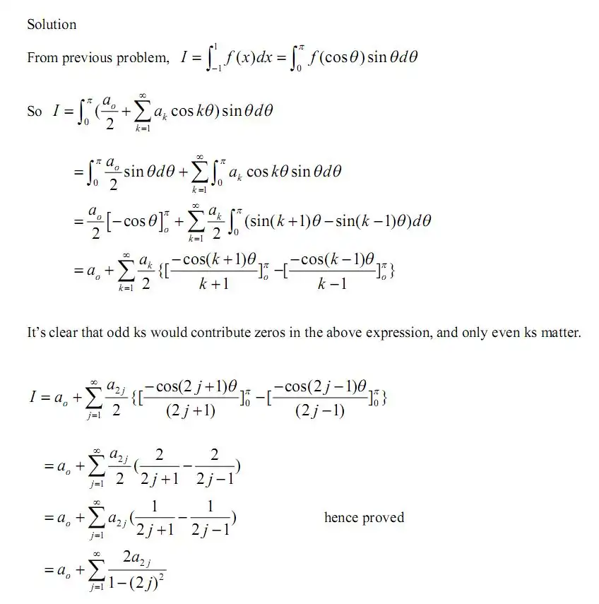
We have the cosine series expressed as , we need to express teh constants as


Solution
We have the given expression for the cosine series as
multiplying both sides by where k is not the same as m and integrating we get,


Using the property of orthogonality we know that exists only when k = m i.e


wkt,
and


Thus we have by substituting and rearranging terms,
Author
--Egm6341.s10.team2.niki 14:43, 23 April 2010 (UTC)
problem15: Expression for Clenshaw-Curtis Quadrature Rule
Statement
Pg.42-3 Simplification of Clenshaw-Curtis Quadrature Rule
Solution
Author
Signatures
solutions of problems 2,7,13,14 --Egm6341.s10.team2.niki 18:48, 23 April 2010 (UTC)
solutions of problems 4,6, 9 --Egm6341.s10.Team2.GV 20:58, 23 April 2010 (UTC)
solutions of problems 1,11,15 --Egm6341.s10.team2.lee 22:47, 23 April 2010 (UTC)
Solution Authors and Reviewers
HW Assignment # 7 | ||
| Problem # | Solution by | Reviewed by |
| Problem 1 | JP | NN |
| Problem 2 | NN | SM |
| Problem 3 | SM | GV |
| Problem 4 | GV | JP |
| Problem 5 | SM | PO |
| Problem 6 | GV | JP |
| Problem 7 | NN & SM | GV |
| Problem 8 | PO | NN |
| Problem 9 | GV | PO |
| Problem 10 | PO | SM |
| Problem 11 | JP | PO |
| Problem 12 | PO | GV |
| Problem 13 | NN | NN |
| Problem 14 | NN | JP |
| Problem 15 | JP | SM |