University of Florida/Eml4507/s13.team4ever.R3

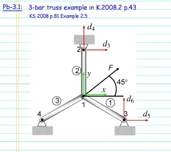
Problem R3.1

Problem Statement

Solution

The following MATLAB program solves for the unknown global displacement DOF's, unknown for components (reactions), and member forces in the system.

function R3_1

F = 20000; %N
E = 206000000000; %Pa
L = 1; %m
A = .0001; %m^2
 
% displacement in meters
d3 = 0.02;  % =u2
d4 = -0.01; % =v2
d5 = -0.03; % =u3
d6 = 0.05;  % =v3

% Table 2.1 KS 2008 p.82
% Element   EA/L      i-->j    phi    l=cos(phi)  m=sin(phi)
% 1       206x10^5    1-->3   -pi/6    0.866       -0.5
% 2       206x10^5    1-->2   -pi/2      0           1
% 3       206x10^5    1-->4   -5pi/6  -0.866       -0.5
 
l1 = 0.866;
m1 = -0.5;
l2 = 0;
m2 = 1;
l3 = -0.866;
m3 = -0.5;
  
% connectivity array
conn = [1 3;1 2;1 4];
 
% location master matrix
lmm = [d1 d2 d5 d6;d1 d2 d3 d4;d1 d2 d7 d8];
 
% element stiffness matrices
% E2.46 
% element 1 stiffness matrix 1-->3
k1 = [l1^2 l1*m1 0 0 -l1^2 -l1*m1 0 0;
      l1*m1 m1^2 0 0 -l1*m1 -m1^2 0 0;
      0 0 0 0 0 0 0 0;
      0 0 0 0 0 0 0 0;
      -l1^2 -l1*m1 0 0 l1^2 l1*m1 0 0;
      -l1*m1 -m1^2 0 0 l1*m1 m1^2 0 0;
      0 0 0 0 0 0 0 0;
      0 0 0 0 0 0 0 0];
  
% element 1 stiffness matrix 1-->2
k2 = [l2^2 l2*m2 -l2^2 -l2*m2 0 0 0 0;
      l2*m2 m2^2 -l2*m2 -m2^2 0 0 0 0;
      -l2^2 -l2*m2 l2^2 l2*m2 0 0 0 0;
      -l2*m2 -m2^2 l2*m2 m2^2 0 0 0 0;
      0 0 0 0 0 0 0 0;
      0 0 0 0 0 0 0 0;
      0 0 0 0 0 0 0 0;
      0 0 0 0 0 0 0 0];
  
% element 1 stiffness matrix 1-->4
k3 = [l3^2 l3*m3 0 0 0 0 -l3^2 -l3*m3;
      l3*m3 m3^2 0 0 0 0 -l3*m3 -m3^2;
      0 0 0 0 0 0 0 0;
      0 0 0 0 0 0 0 0;
      0 0 0 0 0 0 0 0;
      0 0 0 0 0 0 0 0;
      -l3^2 -l3*m3 0 0 0 0 l3^2 l3*m3;
      -l3*m3 -m3^2 0 0 0 0 l3*m3 m3^2];
 
%global stiffness matrix
K = E*A/L*(k1 + k2 + k3);
 
% Force matrix
Fpost = [F*cos(pi/4); F*sin(pi/4); 0; 0; 0; 0; 0; 0];
 

% "forces" of prescribed disp dofs
For=K*d
 
% new force matrix
Fnew = Fpost + For
 
% global disp dofs
disp = K\Fnew

% u2, v2, u3, and v3 are given, so delete rows/columns 3, 4, 7, and 8
Knew = 1*10^7*[3.0898 0 -1.5449 0.8920;
              0 3.0900 0.8920 -0.5150;  
              -1.5449 0.8920 1.5449 -0.8920;
              0.8920 -0.5150 -0.8920 0.5150];

% Force matrix
Fnow = [923600; -304950; -909460; 525090];
 
% displacement values u1, v1, u4, v4 
disp = Knew\Fnow
 
% forces in each element
P1 = E*A/L*(0.866*(d5-disp(1))-0.5*(d6-disp(2)))
P2 = E*A/L*(0*(d3-disp(1))+1*(d4-disp(2)))
P3 = E*A/L*(-0.866*(disp(3)-disp(1))-0.5*(disp(4)-disp(2)))

stress1 = P1/A
stress2 = P2/A
stress3 = P3/A
 

OUTPUT

disp =
    -0.0050
     0.0103
    -0.0257
     0.0764

P1 =
   -854900

P2 =
   -418180

P3 =
   740079

stress1 =
   -8.5490 e009

stress2 =
   -4.1818 e009

stress3 =
   7.4008 e009

Global displacement DOF's (m)
$u_{1}=-0.005$
$v_{1}=-0.0103$
$u_{2}=0.02$
$v_{2}=-0.01$
$u_{3}=-0.03$
$v_{3}=0.05$
$u_{4}=-0.0257$
$v_{4}=0.0764$

Element Reaction Forces (N)
$P^{1}=-854900$
$P^{2}=-418180$
$P^{3}=740079$

Element Stresses (GPa)
$\sigma ^{1}=-8.5490$
$\sigma ^{2}=-4.1818$
$\sigma ^{3}=7.4008$

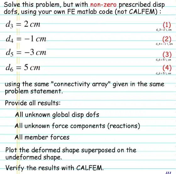
Running a similar MATLAB code using CALFEM verifies the solution

% Checking with CALFEM
edof = [1 1 2 5 6;
        2 1 2 3 4;
        3 1 2 7 8];
 
coord = [cos(pi/4) sin(pi/4);cos(pi/4) 1+sin(pi/4);2*cos(pi/4) 0;0 0];
dof = [1 2;3 4;5 6;7 8];
 
[ex,ey] = coordxtr(edof,coord,dof,2);
ep = [E A];
K = zeros(8);
Fo = zeros(8,1); Fo(1) = F*cos(pi/4); Fo(2) = F*sin(pi/4);
for i = 1:3
    Ke = bar2e(ex(i,:),ey(i,:),ep);
    K = assem(edof(i,:),K,Ke);
end
 
Q = solveq(K,Fo);
ed = extract(edof,Q);
for i = 1:3
    N(i)=bar2s(ex(i,:),ey(i,:),ep,ed(i,:));
end

N1 = N(1)
N2 = N(2)
N3 = N(3)

stress1c = N(1)/A
stress2c = N(2)/A
stress3c = N(3)/A
eldraw2(ex,ey);
grid on


OUTPUT



N1 =
   -8.5490 e005

N2 =
   -4.1818 e005

N3 =
   -7.4008 e005

stress1c =
   -8.5490 e009

stress2c =
   -4.1818 e009

stress3c =
   7.4008 e009

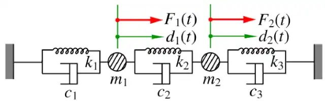
Problem 3.2 Pb-53.5: Draw the FBDs and derive the dif. eq. of motion from p.53-13 (2 DOFs spring-mass-damper system)

On our honor, we did this assignment on our own, without looking at the solutions in previous semesters or other online solutions.

Given a Linearly Elastic Spring-Mass_Damper System With 2 DOFs

Consider a system of three linearly elastic springs and dampers with two masses.

Figure 1: Spring system obtained from EML4507 sec.53.b, Pb-53.5 (Dr. Vu-Quoc) ()

Find:

1.Construct the FBDs for all components

2.Derive the differential equation of motion and the coefficient matrices

$\mathbf {M} {\ddot {\mathbf {d} }}+\mathbf {C} {\dot {\mathbf {d} }}+\mathbf {K} {\mathbf {d} }=\mathbf {F} (t)$

$\mathbf {d} ={\begin{Bmatrix}d_{1}\\d_{2}\end{Bmatrix}}_{2\times 1}$

$\mathbf {F} ={\begin{Bmatrix}F_{1}\\F_{2}\end{Bmatrix}}_{2\times 1}$

$\mathbf {M} ={\begin{bmatrix}m_{1}&0\\0&m_{2}\end{bmatrix}}_{2\times 2}$

$\mathbf {C} ={\begin{bmatrix}(c_{1}+c_{2})&-c_{2}\\-c_{2}&(c_{2}+c_{3})\end{bmatrix}}_{2\times 2}$

$\mathbf {K} ={\begin{bmatrix}(k_{1}+k_{2})&-k_{2}\\-k_{2}&(k_{2}+k_{3})\end{bmatrix}}_{2\times 2}$

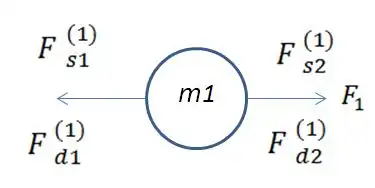
Solution: FBDs of all components

Construct the first FBD (mass 1)

This FBD is of the left mass (mass 1).

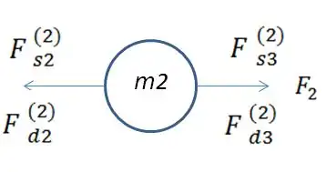
Figure 1: Original Image: FBD of mass 1. ()

Construct the second FBD (mass 2)

This FBD is of the right mass (mass 2).

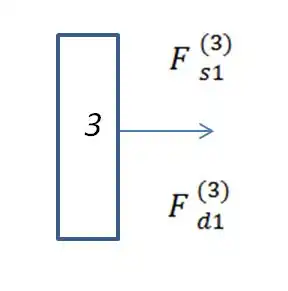
Figure 1: Original Image: FBD of mass 2. ()

Construct the third FBD (left wall support)

This FBD is of the left wall support (item 3).

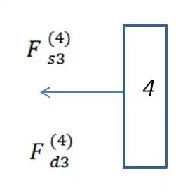
Figure 1: Original Image: FBD of left wall support. ()

Construct the fourth FBD (right wall support)

This FBD is of the right wall support (item 4).

Figure 1: Original Image: FBD of right wall support. ()

Solution: Derive the differential equation of motion and the coefficient matrices

Approach

The position of the masses in the system are described by d1 and d2. The walls are fixed. This means that the values for d3 and d4, for the left and right walls respectively, are zero.

Force Derivations

The springs are assumed to be at their unstretched length (equilibrium) in the figure. A positive d1 causes tension in spring 1 and compression in spring 2. This observation is made from holding m2 stationary. Viewing the last spring from equilibrium, if the mass 2 moves to the right and d2 becomes positive, the third spring will compress.

The differential equations of motion will show that the system is coupled.

$F_{s1}=k_{1}d_{1}$

$F_{d1}=c_{1}{\dot {d}}_{1}$

$F_{s2}=k_{2}(d_{2}-d_{1})$

$F_{d2}=c_{2}({\dot {d}}_{2}-{\dot {d}}_{1})$

$F_{s3}=k_{3}d_{2}$

$F_{d3}=c_{3}{\dot {d}}_{2}$

Summing the Forces

$m_{1}{\ddot {d}}_{1}+(c_{1}+c_{2}){\dot {d}}_{1}-c_{2}{\dot {d}}_{2}+(k_{1}+k_{2})d_{1}-k_{2}d_{2}=F_{1}$

$m_{2}{\ddot {d}}_{2}-c_{2}{\dot {d}}_{1}+(c_{2}+c_{3}){\dot {d}}_{2}-k_{2}d_{1}+(k_{2}+k_{3})d_{2}=F_{2}$

Writing the Two Differential Equations in Matrix Form

Grouping the dependent equations and writing the coefficients in matrix form yields the results shown below.

$\mathbf {M} {\ddot {\mathbf {d} }}+\mathbf {C} {\dot {\mathbf {d} }}+\mathbf {K} {\mathbf {d} }=\mathbf {F} (t)$

$\mathbf {d} ={\begin{Bmatrix}d_{1}\\d_{2}\end{Bmatrix}}_{2\times 1}$

$\mathbf {F} ={\begin{Bmatrix}F_{1}\\F_{2}\end{Bmatrix}}_{2\times 1}$

$\mathbf {M} ={\begin{bmatrix}m_{1}&0\\0&m_{2}\end{bmatrix}}_{2\times 2}$

$\mathbf {C} ={\begin{bmatrix}(c_{1}+c_{2})&-c_{2}\\-c_{2}&(c_{2}+c_{3})\end{bmatrix}}_{2\times 2}$

$\mathbf {K} ={\begin{bmatrix}(k_{1}+k_{2})&-k_{2}\\-k_{2}&(k_{2}+k_{3})\end{bmatrix}}_{2\times 2}$

R3.3

On our Honor, this problem was done without unauthorized help from either solution manuals or other team's reports.
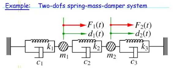
Figure 1: Diagram for Pb-53.6 from page 53-13 in Fead.s13.sec53b lecture notes. Professor Vu-Quoc

Pb-53.6:

Consider the following values for the MDOF system in figure 1 above.
$m_{1}=3,m_{2}=2$
$c_{1}=1/2,c_{2}=1/4,c_{3}=1/3$
$k_{1}=10,k_{2}=20,k_{3}=15$
$F_{1}(t)=0,F_{2}(t)=0$
$d_{1}(0)=-1,d_{2}(0)=2$
$d_{1}'(0)=0,d_{2}'(0)=0$

Problem Statement:

Integrate numerically the governing system L2-ODEs-CC so as to generate the time histories for the disp dofs (The displacement Matrix).

Matlab code showing steps taken to solve problem as discussed in the Fead.s13.sec53b lecture notes p.53-13c-53-13d.

d0=[-1,2];
v0=[0,0];
alpha=1/4; delta=1/2;
nsnap=100;
m1=3;
m2=2;
alpha=1/4; delta=1/2;
d0=[-1,2];
v0=[0,0];
k1=10;
k2=20;
k3=15;
c1=1/2;
c2=1/4;
c3=1/3;
M=[m1,0;0,m2];
C=[(c1+c2),-c2;-c2,(c2+c3)];
K=[(k1+k2),-k2;-k2,(k2+k3)];
[L]=eigen(K,M);
w1=sqrt(L(1));
T1=(2*pi)/w1;
dt=T1/10;
T=[0:dt:5*T1];
Dsnap=step2x(K,C,M,d0,v0,ip,f,pdisp);

EDU>> L
L =
    4.7651
   22.7349
EDU>> w1
w1 =
    2.1829
EDU>> T1
T1 =
    0.3473
EDU>> dt
dt =
    0.0347

Problem R3.4

On my honor, I have neither given nor recieved unauthorized aid in doing this assignment.

Disccription: We are to consider a 1-D bar system with 3 elements. The center element has a known force applied to it's center. Given all information necessary to computed each element stiffness, we are asked to find the displacement at the location of the applied force, as well as the reaction forces at the walls. We are then to verify these results using CALFEM.

Given:

For this problem, we are given that

$E=100*10^{9}$ for all elements

$A_{1}=10^{-4}m^{2}$

$A_{2}=2*10^{-4}m^{2}$

$A_{3}=10^{-4}m^{2}$

$L_{1}=0.3$

$L_{2}=0.4$

$L_{3}=0.3$

The applied force is $F=10,000N$

Solution:

To get the stiffness, we use the equation:

$K={\frac {E*A}{L}}$

Treating this problem as a system with 3 nodes, 2 at the wall and 1 in the center, we need to find the equivalent spring stiffness for each side of the center node. Because the two bars are in series, we can solve for the equivalent K using:

${\frac {1}{K_{eq}}}={\frac {1}{K_{1}}}+{\frac {1}{K_{2}}}$

The following matlab code solves for both the displacement at the center and the reaction forces at the walls.

E = 100*10^9;
A1 = 10^-4;
A2 = 2*10^-4;
L1 = .3;
L2 = .2;
kfirst = E*A1/L1;
ksecond = E*A2/L2;
kinv = (1/kfirst)+(1/ksecond);
k1 = 1/kinv;
k2 = k1;
fsmall = [10000]
ksmall = [0 k1+k2 -k2] 
disp = ksmall\fsmall 
k = [k1 -k1 0;0 k1+k2 -k2;0 -k2 k2] 
F = k*disp

The out from this code yields the following:

disp =

1.0e-003 *

        0
   0.2000
        0

and

F =

      -5000
      10000
      -5000

CALFEM

When then used to verify the above results. The following was the code used for CALFEM:

Edof=[1 1 2;
2 2 3;
3 2 3];

K=zeros(3,3)
f=zeros(3,1);
f(2)=10000
k=25000000;
ep1=k;
ep2=k;
Ke1=spring1e(ep1)
Ke2=spring1e(ep2)
K=assem(Edof(1,:),K,Ke2)
K=assem(Edof(2,:),K,Ke1)

bc= [1 0; 3 0];
[a,r]=solveq(K,f,bc)

This yielded the following results:

a =

 1.0e-003 *

        0
   0.2000
        0

and

r =

      -5000
          0
      -5000

This directly matches our above results, verifying them.

Problem R3.5 Analysis and design of a plane truss

   On my honor, I have neither given nor recieved unauthorized aid in doing this assignment.

Problem Statement

Solution

Input Constants

EDU>> E = 70E9;

EDU>> InL=0.009;

EDU>> OutL=0.012;

EDU>> F = 1000;

Begin Computation of variables

EDU>> InA=InL^2;

EDU>> OutA=OutL^2;

EDU>> A = OutA-InA;

EDU>> L1=sqrt(5);

EDU>> L2=2;

EDU>> K1=E*A/L1;

EDU>> K2=E*A/L2;

EDU>> l=cos(-26.56);

EDU>> m=sin(-26.56);

EDU>> K1a=K1*[l^2 l*m -l^2 -l*m 0 0;

l*m m^2 -l*m -m^2 0 0;

-l^2 -l*m l^2 l*m 0 0;

-l*m -m^2 l*m m^2 0 0;

0 0 0 0 0 0;

0 0 0 0 0 0];

EDU>> K2a = K2*[0 0 0 0 0 0;

0 0 0 0 0 0;

0 0 1 0 -1 0;

0 0 0 0 0 0;

0 0 -1 0 1 0;

0 0 0 0 0 0];

Cut down matrices to do calculations

EDU>> A = [K(3,:);K(4,:)]

A =

  1.0e+06 *

 Columns 1 through 4

  -0.0404    0.2792    2.2454   -0.2792
   0.2792   -1.9319   -0.2792    1.9319

 Columns 5 through 6

  -2.2050         0
        0         0

EDU>> B = [A(:,3) A(:,4)]

B =

  1.0e+06 *

   2.2454   -0.2792
  -0.2792    1.9319

EDU>> Fa = [0;-1000];

Final Results from Matlab

EDU>> d = B\Fa

d =

  1.0e-03 *

  -0.0655
  -0.5271

EDU>> d1=[0;0;d(1);d(2);0;0]

d1 =

  1.0e-03 *

Reaction Forces

EDU>> F = K*d1

F =

  1.0e+03 *

Comparing to yield strength and buckling force

To test the member in tension

$\sigma ={\frac {F}{A}}$ $\sigma ={\frac {1010N}{6.3*10^{-5}m^{2}}}=16.03MPa$

The stress is well under the yield strength so this value is fine.

====To test the member in compression $P_{cr}={\frac {\pi ^{2}EI}{L}}$ $P_{cr}={\frac {\pi ^{2}(70*10^{9})*(1.18*10^{-9})}{2}}=408.4N$

We can compare this to the actually force of 144.5 N.

Optimize

To optimize for the lowest weight while still being safe, we can turn the above matlab program into an .m file and adjust the dimensions of the cross section. When optimized, the outer member will be 12mm and inner hole will be 10.5mm.

EDU>> [u v]=Report3(0.012,0.0105)

u =

  1.0e+03 *

v =

 247.0138

For the above calculation, u is the stress in each member and v is P critical for bending. This is well within the range to not buckle with a factor of safety of 1.2 and the tensile stress is also well within the factor of safety of 2.

Calfem Verification

EDU>> A = 0.012^2-0.009^2;

EDU>> E = 70E9;

EDU>> Edof = [1 1 2 3 4;

2 3 4 5 6];

EDU>> K = zeros(6);

EDU>> f = zeros(6,1);

EDU>> f (4) = -1000;

EDU>> ep = [E A];

EDU>> Ex = [0 2;

2 0];

EDU>> Ey = [1 0;

0 0];

EDU>> for i = 1:2

Ke = bar2e(Ex(i,:),Ey(i,:),ep);

K = assem(Edof(i,:),K,Ke);

end;

EDU>> bc = [1 0;2 0;5 0;6 0];

EDU>> [a,r]=solveq(K,f,bc)

a =

r =

  1.0e+03 *

When verified with calfem, the reactions didn't match the numbers from matlab or hand calculations. The displacement seems to be closer to what would be expected in real life applications however the reaction forces seem strange. We were not able to find the cause for this error.

Problem 3.6 Determine Truss System Deformation

On my honor, I have neither given nor recieved unauthorized aid in doing this assignment.

Problem Statement

Analyze a plane truss from figure 2.28 of KS2008 pg. 96.

Solution

The nodal numbers displayed in fig. 2.28 for the following solutions are numbered horizontally along the bottom of the truss, and then along the top.

Input Constants

Part 1 Find the Deflections and Element Forces

Case A

EDU>> Edof=[1 1 2 3 4;2 3 4 5 6; 3 5 6 7 8;4 7 8 9 10;5 9 10 11 12; 6 11 12 13

14; 7 15 16 17 18;8 17 18 19 20;9 19 20 21 22; 10 21 22 23 24; 11 23 24 25 26;

12 25 26 27 28; 13 1 2 15 16;14 3 4 17 18; 15 5 6 19 20;16 7 8 21 22;17 9 10 23

24; 18 11 12 25 26; 19 13 14 27 28; 20 1 2 17 18; 21 3 4 19 20; 22 5 6 21 22; 23

7 8 23 24;24 9 10 25 26;25 11 12 27 28];

EDU>> L = 0.3;

EDU>> E = 100000000000;

EDU>> A = 0.0001;

EDU>> L2 = L*sqrt(2);

EDU>> K = zeros(28);

EDU>> f = zeros(28,1);

EDU>> f(13) = 10000; f(27) = 10000;

EDU>> ep = [E A];

EDU>> Ex = [0 L; L 2*L; 2*L 3*L;3*L 4*L; 4*L 5*L;5*L 6*L;0 L; L 2*L; 2*L 3*L;3*L 4*L; 4*L 5*L;5*L 6*L;0 0; L L; 2*L 2*L;3*L 3*L;4*L 4*L;5*L 5*L;6*L 6*L;0 L; L 2*L; 2*L 3*L;3*L 4*L; 4*L 5*L;5*L 6*L];

EDU>> Ey = [0 0;0 0;0 0;0 0;0 0;0 0;L L;L L;L L;L L;L L;L L;0 L;0 L;0 L;0 L;0 L;0 L;0 L;0 L;0 L;0 L;0 L;0 L;0 L];

EDU>> for i = 1:25

Ke = bar2e(Ex(i,:),Ey(i,:),ep);

K = assem(Edof(i,:),K,Ke);

end;

EDU>> bc = [1 0;2 0;15 0;16 0];

EDU>> [a,r]=solveq(K,f,bc)

a =

r =

  1.0e+04 *

Case B

EDU>> Edof=[1 1 2 3 4;2 3 4 5 6; 3 5 6 7 8;4 7 8 9 10;5 9 10 11 12; 6 11 12 13 14; 7 15 16 17 18;8 17 18 19 20;9 19 20 21 22; 10 21 22 23 24; 11 23 24 25 26; 12 25 26 27 28; 13 1 2 15 16;14 3 4 17 18; 15 5 6 19 20;16 7 8 21 22;17 9 10 23 24; 18 11 12 25 26; 19 13 14 27 28; 20 1 2 17 18; 21 3 4 19 20; 22 5 6 21 22; 23 7 8 23 24;24 9 10 25 26;25 11 12 27 28];

EDU>> L = 0.3;

EDU>> E = 100000000000;

EDU>> A = 0.0001;

EDU>> L2 = L*sqrt(2);

EDU>> K = zeros(28);

EDU>> f = zeros(28,1);

EDU>> f(14) = 10000; f(28) = 10000;

EDU>> ep = [E A];

EDU>> Ex = [0 L; L 2*L; 2*L 3*L;3*L 4*L; 4*L 5*L;5*L 6*L;0 L; L 2*L; 2*L 3*L;3*L 4*L; 4*L 5*L;5*L 6*L;0 0; L L; 2*L 2*L;3*L 3*L;4*L 4*L;5*L 5*L;6*L 6*L;0 L; L 2*L; 2*L 3*L;3*L 4*L; 4*L 5*L;5*L 6*L];

EDU>> Ey = [0 0;0 0;0 0;0 0;0 0;0 0;L L;L L;L L;L L;L L;L L;0 L;0 L;0 L;0 L;0 L;0 L;0 L;0 L;0 L;0 L;0 L;0 L;0 L];

EDU>> for i = 1:25

Ke = bar2e(Ex(i,:),Ey(i,:),ep);

K = assem(Edof(i,:),K,Ke);

end;

EDU>> bc = [1 0;2 0;15 0;16 0];

EDU>> [a,r]=solveq(K,f,bc)

a =

r =

  1.0e+05 *

Case c

EDU>> Edof=[1 1 2 3 4;2 3 4 5 6; 3 5 6 7 8;4 7 8 9 10;5 9 10 11 12; 6 11 12 13 14; 7 15 16 17 18;8 17 18 19 20;9 19 20 21 22; 10 21 22 23 24; 11 23 24 25 26; 12 25 26 27 28; 13 1 2 15 16;14 3 4 17 18; 15 5 6 19 20;16 7 8 21 22;17 9 10 23 24; 18 11 12 25 26; 19 13 14 27 28; 20 1 2 17 18; 21 3 4 19 20; 22 5 6 21 22; 23 7 8 23 24;24 9 10 25 26;25 11 12 27 28];

EDU>> L = 0.3;

EDU>> E = 100000000000;

EDU>> A = 0.0001;

EDU>> L2 = L*sqrt(2);

EDU>> K = zeros(28);

EDU>> f = zeros(28,1);

EDU>> f(13) = 10000; f(27) = -10000;

EDU>> ep = [E A];

EDU>> Ex = [0 L; L 2*L; 2*L 3*L;3*L 4*L; 4*L 5*L;5*L 6*L;0 L; L 2*L; 2*L 3*L;3*L 4*L; 4*L 5*L;5*L 6*L;0 0; L L; 2*L 2*L;3*L 3*L;4*L 4*L;5*L 5*L;6*L 6*L;0 L; L 2*L; 2*L 3*L;3*L 4*L; 4*L 5*L;5*L 6*L];

EDU>> Ey = [0 0;0 0;0 0;0 0;0 0;0 0;L L;L L;L L;L L;L L;L L;0 L;0 L;0 L;0 L;0 L;0 L;0 L;0 L;0 L;0 L;0 L;0 L;0 L];

EDU>> for i = 1:25

Ke = bar2e(Ex(i,:),Ey(i,:),ep);

K = assem(Edof(i,:),K,Ke);

end;

EDU>> bc = [1 0;2 0;15 0;16 0];

EDU>> [a,r]=solveq(K,f,bc)

a =

r =

  1.0e+04 *

Part 3 Verify the Beam Model Adding 2 Bays...

Case A

EDU>> Edof=[1 1 2 3 4;2 3 4 5 6; 3 5 6 7 8;4 7 8 9 10;5 9 10 11 12; 6 11 12 13 14; 7 13 14 15 16; 8 15 16 17 18; 9 19 20 21 22; 10 21 22 23 24; 11 23 24 25 26; 12 25 26 27 28; 13 27 28 29 30; 14 29 30 31 32; 15 31 32 33 34; 16 33 34 35 36; 17 1 2 19 20;18 3 4 21 22; 19 5 6 23 24; 20 7 8 25 26; 21 9 10 27 28; 22 11 12 29 30; 23 13 14 31 32; 24 15 16 33 34; 25 17 18 35 36; 26 1 2 21 22; 27 3 4 23 24; 28 5 6 25 26; 29 7 8 27 28; 30 9 10 29 30; 31 11 12 31 32; 32 13 14 33 34; 33 15 16 35 36]

Edof =

    1     1     2     3     4
    2     3     4     5     6
    3     5     6     7     8
    4     7     8     9    10
    5     9    10    11    12
    6    11    12    13    14
    7    13    14    15    16
    8    15    16    17    18
    9    19    20    21    22
   10    21    22    23    24
   11    23    24    25    26
   12    25    26    27    28
   13    27    28    29    30
   14    29    30    31    32
   15    31    32    33    34
   16    33    34    35    36
   17     1     2    19    20
   18     3     4    21    22
   19     5     6    23    24
   20     7     8    25    26
   21     9    10    27    28
   22    11    12    29    30
   23    13    14    31    32
   24    15    16    33    34
   25    17    18    35    36
   26     1     2    21    22
   27     3     4    23    24
   28     5     6    25    26
   29     7     8    27    28
   30     9    10    29    30
   31    11    12    31    32
   32    13    14    33    34
   33    15    16    35    36

EDU>> L = 0.3;

EDU>> E = 100000000000;

EDU>> A = 0.0001;

EDU>> L2 = L*sqrt(2);

EDU>> K = zeros(36);

EDU>> f = zeros(36,1);

EDU>> f(17) = 10000; f(35) = 10000;

EDU>> ep = [E A];

EDU>> Ex = [0 L; L 2*L; 2*L 3*L;3*L 4*L; 4*L 5*L;5*L 6*L;6*L 7*L;7*L 8*L;0 L; L 2*L; 2*L 3*L;3*L 4*L; 4*L 5*L;5*L 6*L;6*L 7*L;7*L 8*L;0 0; L L; 2*L 2*L;3*L 3*L;4*L 4*L;5*L 5*L;6*L 6*L;7*L 7*L;8*L 8*L;0 L; L 2*L; 2*L 3*L;3*L 4*L; 4*L 5*L;5*L 6*L;6*L 7*L;7*L 8*L];

EDU>> Ey = [0 0;0 0;0 0;0 0;0 0;0 0;0 0;0 0;L L;L L;L L;L L;L L;L L;L L;L L;0 L;0 L;0 L;0 L;0 L;0 L;0 L;0 L;0 L;0 L;0 L;0 L;0 L;0 L;0 L;0 L;0 L];

EDU>> for i = 1:33

Ke = bar2e(Ex(i,:),Ey(i,:),ep);

K = assem(Edof(i,:),K,Ke);

end;

EDU>> bc = [1 0;2 0;19 0;20 0];

EDU>> [a,r]=solveq(K,f,bc)

a =

r =

  1.0e+04 *

Case B

EDU>> Edof=[1 1 2 3 4;2 3 4 5 6; 3 5 6 7 8;4 7 8 9 10;5 9 10 11 12; 6 11 12 13 14; 7 13 14 15 16; 8 15 16 17 18; 9 19 20 21 22; 10 21 22 23 24; 11 23 24 25 26; 12 25 26 27 28; 13 27 28 29 30; 14 29 30 31 32; 15 31 32 33 34; 16 33 34 35 36; 17 1 2 19 20;18 3 4 21 22; 19 5 6 23 24; 20 7 8 25 26; 21 9 10 27 28; 22 11 12 29 30; 23 13 14 31 32; 24 15 16 33 34; 25 17 18 35 36; 26 1 2 21 22; 27 3 4 23 24; 28 5 6 25 26; 29 7 8 27 28; 30 9 10 29 30; 31 11 12 31 32; 32 13 14 33 34; 33 15 16 35 36]

Edof =

    1     1     2     3     4
    2     3     4     5     6
    3     5     6     7     8
    4     7     8     9    10
    5     9    10    11    12
    6    11    12    13    14
    7    13    14    15    16
    8    15    16    17    18
    9    19    20    21    22
   10    21    22    23    24
   11    23    24    25    26
   12    25    26    27    28
   13    27    28    29    30
   14    29    30    31    32
   15    31    32    33    34
   16    33    34    35    36
   17     1     2    19    20
   18     3     4    21    22
   19     5     6    23    24
   20     7     8    25    26
   21     9    10    27    28
   22    11    12    29    30
   23    13    14    31    32
   24    15    16    33    34
   25    17    18    35    36
   26     1     2    21    22
   27     3     4    23    24
   28     5     6    25    26
   29     7     8    27    28
   30     9    10    29    30
   31    11    12    31    32
   32    13    14    33    34
   33    15    16    35    36

EDU>> L = 0.3;

EDU>> E = 100000000000;

EDU>> A = 0.0001;

EDU>> L2 = L*sqrt(2);

EDU>> K = zeros(36);

EDU>> f = zeros(36,1);

EDU>> f(18) = 10000; f(36) = 10000;

EDU>> ep = [E A];

EDU>> Ex = [0 L; L 2*L; 2*L 3*L;3*L 4*L; 4*L 5*L;5*L 6*L;6*L 7*L;7*L 8*L;0 L; L 2*L; 2*L 3*L;3*L 4*L; 4*L 5*L;5*L 6*L;6*L 7*L;7*L 8*L;0 0; L L; 2*L 2*L;3*L 3*L;4*L 4*L;5*L 5*L;6*L 6*L;7*L 7*L;8*L 8*L;0 L; L 2*L; 2*L 3*L;3*L 4*L; 4*L 5*L;5*L 6*L;6*L 7*L;7*L 8*L];

EDU>> Ey = [0 0;0 0;0 0;0 0;0 0;0 0;0 0;0 0;L L;L L;L L;L L;L L;L L;L L;L L;0 L;0 L;0 L;0 L;0 L;0 L;0 L;0 L;0 L;0 L;0 L;0 L;0 L;0 L;0 L;0 L;0 L];

EDU>> for i = 1:33

Ke = bar2e(Ex(i,:),Ey(i,:),ep);

K = assem(Edof(i,:),K,Ke);

end;

EDU>> bc = [1 0;2 0;19 0;20 0];

EDU>> [a,r]=solveq(K,f,bc)

a =

r =

  1.0e+05 *

Case C

EDU>> Edof=[1 1 2 3 4;2 3 4 5 6; 3 5 6 7 8;4 7 8 9 10;5 9 10 11 12; 6 11 12 13 14; 7 13 14 15 16; 8 15 16 17 18; 9 19 20 21 22; 10 21 22 23 24; 11 23 24 25 26; 12 25 26 27 28; 13 27 28 29 30; 14 29 30 31 32; 15 31 32 33 34; 16 33 34 35 36; 17 1 2 19 20;18 3 4 21 22; 19 5 6 23 24; 20 7 8 25 26; 21 9 10 27 28; 22 11 12 29 30; 23 13 14 31 32; 24 15 16 33 34; 25 17 18 35 36; 26 1 2 21 22; 27 3 4 23 24; 28 5 6 25 26; 29 7 8 27 28; 30 9 10 29 30; 31 11 12 31 32; 32 13 14 33 34; 33 15 16 35 36]

Edof =

    1     1     2     3     4
    2     3     4     5     6
    3     5     6     7     8
    4     7     8     9    10
    5     9    10    11    12
    6    11    12    13    14
    7    13    14    15    16
    8    15    16    17    18
    9    19    20    21    22
   10    21    22    23    24
   11    23    24    25    26
   12    25    26    27    28
   13    27    28    29    30
   14    29    30    31    32
   15    31    32    33    34
   16    33    34    35    36
   17     1     2    19    20
   18     3     4    21    22
   19     5     6    23    24
   20     7     8    25    26
   21     9    10    27    28
   22    11    12    29    30
   23    13    14    31    32
   24    15    16    33    34
   25    17    18    35    36
   26     1     2    21    22
   27     3     4    23    24
   28     5     6    25    26
   29     7     8    27    28
   30     9    10    29    30
   31    11    12    31    32
   32    13    14    33    34
   33    15    16    35    36

EDU>> L = 0.3;

EDU>> E = 100000000000;

EDU>> A = 0.0001;

EDU>> L2 = L*sqrt(2);

EDU>> K = zeros(36);

EDU>> f = zeros(36,1);

EDU>> f(17) = 10000; f(35) = -10000;

EDU>> ep = [E A];

EDU>> Ex = [0 L; L 2*L; 2*L 3*L;3*L 4*L; 4*L 5*L;5*L 6*L;6*L 7*L;7*L 8*L;0 L; L 2*L; 2*L 3*L;3*L 4*L; 4*L 5*L;5*L 6*L;6*L 7*L;7*L 8*L;0 0; L L; 2*L 2*L;3*L 3*L;4*L 4*L;5*L 5*L;6*L 6*L;7*L 7*L;8*L 8*L;0 L; L 2*L; 2*L 3*L;3*L 4*L; 4*L 5*L;5*L 6*L;6*L 7*L;7*L 8*L];

EDU>> Ey = [0 0;0 0;0 0;0 0;0 0;0 0;0 0;0 0;L L;L L;L L;L L;L L;L L;L L;L L;0 L;0 L;0 L;0 L;0 L;0 L;0 L;0 L;0 L;0 L;0 L;0 L;0 L;0 L;0 L;0 L;0 L];

EDU>> for i = 1:33

Ke = bar2e(Ex(i,:),Ey(i,:),ep);

K = assem(Edof(i,:),K,Ke);

end;

EDU>> bc = [1 0;2 0;19 0;20 0];

EDU>> [a,r]=solveq(K,f,bc)

a =

r =

  1.0e+03 *

Problem 3.7 Verify Stiffness matrix

On my honor, I have neither given nor recieved unauthorized aid in doing this assignment.

Given Equations

Given the two following equations, verify that they simplify to the bar element stiffness matrix ${\bar {k}}^{(e)}$ .

$\mathbf {1} )$ ${\bar {k}}^{(e)}=T^{(e)T}{\hat {k}}^{(e)}T^{(e)}$

$\mathbf {2} )$ ${\bar {k}}^{(e)}={\widetilde {T}}^{{(e)}T}\,{\widetilde {k}}^{(e)}\,{\widetilde {T}}^{(e)}$

Solution 1

Original Equation

${\bar {k}}^{(e)}=T^{(e)T}{\hat {k}}^{(e)}T^{(e)}$

Given Equations

${\hat {k}}^{(e)}=k^{(e)}{\begin{bmatrix}1&-1\\-1&1\end{bmatrix}}={\begin{bmatrix}k^{(e)}&-k^{(e)}\\-k^{(e)}&k^{(e)}\end{bmatrix}}$

$T^{(e)}={\begin{bmatrix}l^{(e)}&m^{(e)}&0&0\\0&0&l^{(e)}&m^{(e)}\end{bmatrix}}$

Plugging into original Equation

${\bar {k}}^{(e)}={\begin{bmatrix}l^{(e)}&0\\m^{(e)}&0\\0&l^{(e)}\\0&m^{(e)}\end{bmatrix}}{\begin{bmatrix}k^{(e)}&-k^{(e)}\\-k^{(e)}&k^{(e)}\end{bmatrix}}{\begin{bmatrix}l^{(e)}&m^{(e)}&0&0\\0&0&l^{(e)}&m^{(e)}\end{bmatrix}}$

Solving

Multiple the first two equations. ${\bar {k}}^{(e)}={\begin{bmatrix}l^{(e)}k^{(e)}&-l^{(e)}k^{(e)}\\m^{(e)}k^{(e)}&-m^{(e)}k^{(e)}\\-l^{(e)}k^{(e)}&l^{(e)}k^{(e)}\\-m^{(e)}k^{(e)}&m^{(e)}k^{(e)}\end{bmatrix}}{\begin{bmatrix}l^{(e)}&m^{(e)}&0&0\\0&0&l^{(e)}&m^{(e)}\end{bmatrix}}$

Pull out the K term. ${\bar {k}}^{(e)}=k^{(e)}{\begin{bmatrix}l^{(e)}&-l^{(e)}\\m^{(e)}&-m^{(e)}\\-l^{(e)}&l^{(e)}\\-m^{(e)}&m^{(e)}\end{bmatrix}}{\begin{bmatrix}l^{(e)}&m^{(e)}&0&0\\0&0&l^{(e)}&m^{(e)}\end{bmatrix}}$

Multiple the last two matrices to get the following equation: ${\bar {k}}^{(e)}=k^{(e)}{\begin{bmatrix}l^{(e)2}&l^{(e)}m^{(e)}&-l^{(e)2}&-l^{(e)}m^{(e)}\\l^{(e)}m^{(e)}&m^{(e)2}&-l^{(e)}m^{(e)}&-m^{(e)2}\\-l^{(e)2}&-l^{(e)}m^{(e)}&l^{(e)2}&l^{(e)}m^{(e)}\\-l^{(e)}m^{(e)}&-m^{(e)2}&l^{(e)}m^{(e)}&m^{(e)2}\end{bmatrix}}$

This shows that the original equation can be simplified down to the bar element stiffness matrix.

Solution 2

Original Equation

$k^{(e)}={\widetilde {T}}^{{(e)}T}\,{\widetilde {k}}^{(e)}\,{\widetilde {T}}^{(e)}$

Provided equations

${\widetilde {T}}^{(e)}={\begin{bmatrix}cos(\phi )&sin(\phi )&0&0\\-sin(\phi )&cos(\phi )&0&0\\0&0&cos(\phi )&sin(\phi )\\0&0&-sin(\phi )&cos(\phi )\end{bmatrix}}$

${\widetilde {k}}^{(e)}={\frac {EA}{L}}{\begin{bmatrix}1&0&-1&0\\0&0&0&0\\-1&0&1&0\\0&0&0&0\end{bmatrix}}$

Plugging into Original Equation

$k^{(e)}={\begin{bmatrix}cos(\phi )&-sin(\phi )&0&0\\sin(\phi )&cos(\phi )&0&0\\0&0&cos(\phi )&-sin(\phi )\\0&0&sin(\phi )&cos(\phi )\end{bmatrix}}{\frac {EA}{L}}{\begin{bmatrix}1&0&-1&0\\0&0&0&0\\-1&0&1&0\\0&0&0&0\end{bmatrix}}{\begin{bmatrix}cos(\phi )&sin(\phi )&0&0\\-sin(\phi )&cos(\phi )&0&0\\0&0&cos(\phi )&sin(\phi )\\0&0&-sin(\phi )&cos(\phi )\end{bmatrix}}$

Solving

Begin by multiplying the first two matrices together. $k^{(e)}={\frac {EA}{L}}{\begin{bmatrix}cos(\phi )&0&-cos(\phi )&0\\sin(\phi )&0&-sin(\phi )&0\\-cos(\phi )&0&cos(\phi )&0\\-sin(\phi )&0&sin(\phi )&0\end{bmatrix}}{\begin{bmatrix}cos(\phi )&sin(\phi )&0&0\\-sin(\phi )&cos(\phi )&0&0\\0&0&cos(\phi )&sin(\phi )\\0&0&-sin(\phi )&cos(\phi )\end{bmatrix}}$

Next, multiply the last two together. $k^{(e)}={\frac {EA}{L}}{\begin{bmatrix}cos(\phi )^{2}&cos(\phi )sin(\phi )&-cos(\phi )^{2}&-cos(\phi )sin(\phi )\\cos(\phi )sin(\phi )&sin(\phi )^{2}&-cos(\phi )sin(\phi )&-sin(\phi )^{2}\\-cos(\phi )^{2}&-cos(\phi )sin(\phi )&cos(\phi )^{2}&cos(\phi )sin(\phi )\\cos(\phi )sin(\phi )&-sin(\phi )^{2}&-cos(\phi )sin(\phi )&sin(\phi )^{2}\end{bmatrix}}$

This verifies our original expectation that the equation would simplify down to the bar element stiffness matrix.

Problem R3.8

   On my honor, I have neither given nor recieved unauthorized aid in doing this assignment.

We are asked to redo problem R2.4

Description: We are to find an expression for the excitation referenced in (1) p.53-6 and then find the actual solution and the amplification factor, A for the following conditions:

$f_{0}/m=r_{0}=1$
${\bar {w}}=0.9w$

We are then to find the complete solution.

Solution:

$y''+y'+({\frac {17}{4}})y={\frac {f_{0}}{m}}cos({\bar {w}}t)$

Let us guess the solution is:

$y_{p}(t)=Asin({\bar {w}}t)+Bcos({\bar {w}}t)$

then

$y_{p}(t)=Asin({\bar {w}}t)+Bcos({\bar {w}}t)$
$y'_{p}(t)=A{\bar {w}}cos({\bar {w}}t)-B{\bar {w}}sin({\bar {w}}t)$
$y''_{p}(t)=-A{\bar {w}}^{2}cos({\bar {w}}t)-B{\bar {w}}^{2}sin({\bar {w}}t)$

We then write

$[-A{\bar {w}}^{2}-B{\bar {w}}+({\frac {17}{4}})A]sin({\bar {w}}t)+[-B{\bar {w}}^{2}+A{\bar {w}}+({\frac {17}{4}})B]cos({\bar {w}}t)={\frac {f_{0}}{m}}cos({\bar {w}}t)$

It follows that

$[-A{\bar {w}}^{2}-B{\bar {w}}+({\frac {17}{4}})A]=0$ and that $[-B{\bar {w}}^{2}+A{\bar {w}}+({\frac {17}{4}})B]={\frac {f_{0}}{m}}$

We solve for A and B to be

$A={\frac {f_{0}/m}{[{\bar {w}}+({\frac {17}{4}})^{2}({\frac {1}{\bar {w}}})-{\frac {34{\bar {w}}}{4}}+{\bar {w}}^{3}]}}$
$B={\frac {{\frac {f_{0}}{m}}[{\frac {17}{4}}-{\bar {w}}^{2}]}{[[{\bar {w}}+({\frac {17}{4}})^{2}({\frac {1}{\bar {w}}})-{\frac {34{\bar {w}}}{4}}+{\bar {w}}^{3}]({\bar {w}})]}}$

Once given the conditions

$f_{0}/m=r_{0}=1$
${\bar {w}}=0.9w$

we can find

${\bar {w}}=0.9w={\bar {w}}=0.9*2.0615=1.855$

Plugging these values in yields

$A=0.4528$
$B=0.1975$

The particular solution is then

$y_{p}(t)=0.4528sin(1.855t)+0.1975cos(1.855t)$

Equations (3) p. 53-8 and (2) p. 53-8 give us

$\rho ={\frac {\bar {w}}{w}}={\frac {1.855}{2.0615}}=0.9$
$A={\frac {1}{[(1-\rho ^{2})^{2}+(2\zeta \rho )^{2}]^{\frac {1}{2}}}}={\frac {1}{[(1-0.9^{2})^{2}+(2*0.2425*0.9)^{2}]^{\frac {1}{2}}}}=2.1006$

We then need to find the total solution given the boundary conditions from R2.4; http://en.wikiversity.org/wiki/Fead-s13-team4-R2#Solution

We have for the homogeneous solution from R1.5:

$y_{h}=Ae^{-0.5t}cos(2t)+Be^{-0.5t}sin(2t)$

The total solution can then be found from

$y(t)=y_{h}+y_{p}$

We have then for the total solution:

$y(t)=Ae^{-0.5t}cos(2t)+Be^{-0.5t}sin(2t)+0.4528sin(1.855t)+0.1975cos(1.855t)$

We now need to find the coefficients A and B using the initial conditions:

$y(0)=1$ and $y'(0)=0$

Taking the derivative of y(t), we obtain:

$y'(t)=-0.5Ae^{-1.5t}cos(2t)-2Ae^{-0.5t}sin(2t)-0.5Be^{-1.5t}sin(2t)+2Be^{-0.5t}cos(2t)+0.8399cos(1.855t)-0.3663sin(1.855t)$

Plugging in t = 0 for both the equation of y(t) and y'(t) allows us to find the values of A and B.

From the equation for y(t):

$A(1)+0.1975=1$

$A=0.8025$

From the equation for y'(t):

$-0.5A+2B+0.8399=0$

$2B=-0.8399+0.5*0.8024=-0.4386$

$B=-0.2193$

Hence, the total solution is:

$y(t)=0.8025e^{-0.5t}cos(2t)-0.2193e^{-0.5t}sin(2t)+0.4528sin(1.855t)+0.1975cos(1.855t)$

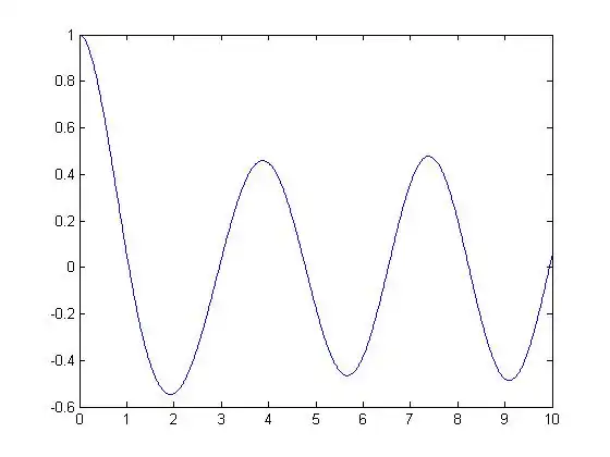
The following is the graph of the homogeneous solution:

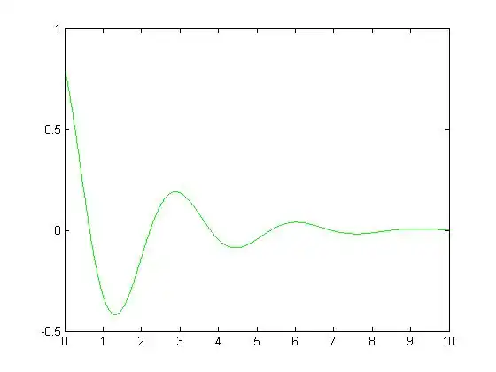
The following is the graph of the particular solution:

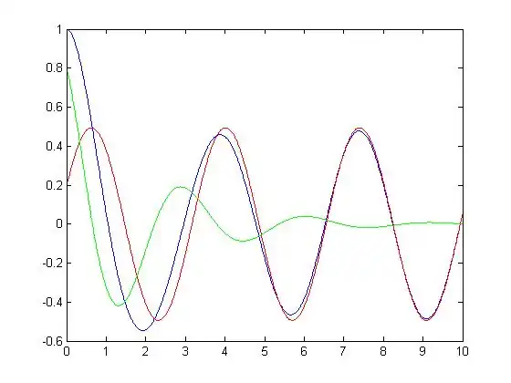
The following is the graph of the total solution, $y(t)=y_{h}(t)+y_{p}(t)$ :

A graph of all three plots is produced below:

Contribution

Problem Assignments
Problem #	Solved&Typed by	Reviewed by
1	Chad Colocar, Bryan Tobin	All
2	Vernon Babich, Tyler Wulterkens	All
3	Bryan Tobin, Chad Colocar	All
4	David Bonner, Vernon Babich	All
5	Was Dean Pickett, David Bonner	All
6	Was Dean Pickett, Tyler Wulterkens	All
7	Tyler Wulterkens, David Bonner	All
8	David Bonner, Vernon Babich	All

This article is issued from Wikiversity. The text is licensed under Creative Commons - Attribution - Sharealike. Additional terms may apply for the media files.