University of Florida/Eml4507/s13.team4ever.Wulterkens.R2
Problem 2.1 Model 2-D Truss With 2 Inclined Elements and Verify Assembly
Given 2-D Truss Model and Constants
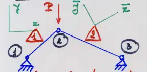
Consider the 2D truss system
Use the following constants to very calculations


Find:
1) Explain the Assembly Process of the Above 2D Truss System
2) Verify With CALFEM
Solution: Assembly Process for 2d Truss System
Construct local stiffness matrices
The stiffness matrices will be constructed for individual elements 1 and 2. The rows and columns will be numbered to represent the force and degree of freedom. For element 1

For element 2

The variable K can be determined by

If the variables are plugged in, we get the following matrices:
For element 1

For element 2

It is clear that if we wish to combine the matrices, it will place coordinate 3,3 of element 2 on the location of 3,3 of element 1 due to them referencing the same point in the same direction. When combining the matrices, addition will be used since the matrices represent directional forces and forces always combine in the same direction by addition.
Combining local stiffness matrices into a global matrix
The local matrices from element 1 and 2 will be combined as described above to give

Solution: Verify With CALFEM
MatLab Code
EDU>> Edof = [1 1 2 3 4
2 3 4 5 6];
EDU>> K = zeros(6);
EDU>> f = zeros(6,1);
EDU>> f(4) = -7;
EDU>> E1 = 3; E2 = 5;
EDU>> L1 = 4;L2 = 2;
EDU>> A1 = 1;A2 = 2;
EDU>> ep1 = [E1 A1]
ep1 =
3 1
EDU>> ep2 = [E2 A2]
ep2 =
5 2
EDU>> ex1 = [-3.464 0]; ex2 = [0 1.414];
EDU>> ey1 = [-2 0]; ey2 = [0 -1.414];
EDU>> Ke1 = bar2e(ex1,ey1,ep1)
Ke1 =
   0.5625    0.3248   -0.5625   -0.3248
   0.3248    0.1875   -0.3248   -0.1875
  -0.5625   -0.3248    0.5625    0.3248
  -0.3248   -0.1875    0.3248    0.1875
EDU>> Ke2 = bar2e(ex2,ey2,ep2)
Ke2 =
   2.5004   -2.5004   -2.5004    2.5004
  -2.5004    2.5004    2.5004   -2.5004
  -2.5004    2.5004    2.5004   -2.5004
   2.5004   -2.5004   -2.5004    2.5004
EDU>> K = assem(Edof(1,:),K,Ke1);
EDU>> K = assem(Edof(2,:),K,Ke2)
K =
   0.5625    0.3248   -0.5625   -0.3248         0         0
   0.3248    0.1875   -0.3248   -0.1875         0         0
  -0.5625   -0.3248    3.0629   -2.1756   -2.5004    2.5004
  -0.3248   -0.1875   -2.1756    2.6879    2.5004   -2.5004
        0         0   -2.5004    2.5004    2.5004   -2.5004
        0         0    2.5004    -2.5004  -2.5004    2.5004
EDU>> bc = [1 0;2 0;5 0;6 0];
EDU>> [a,r]=solveq(K,f,bc)
a =
        0
        0
  -4.3519
  -6.1268
        0
        0
r =
   4.4378
   2.5622
        0
  -0.0000
  -4.4378
   4.4378
Conclusion
By comparing the value from the hand calculation and the value from the CALFEM program, we can see that the two matrices are identical. This verifies the assembly process of using addition when combining local matrices by addition.
--EML4507.s13.team4ever.Wulterkens (discuss • contribs) 07:21, 6 February 2013 (UTC)