3

In PPO with clipped surrogate objective (see the paper here), we have the following objective:

PPO objective

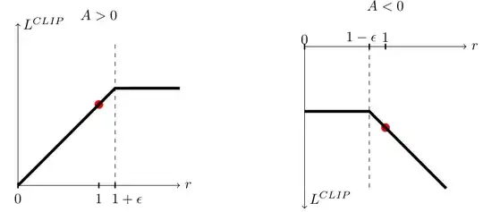
The shape of the function is shown in the image below, and depends on whether the advantage is positive or negative.

objective plot over r

The min() operator makes $L^{CLIP}(\theta)$ a lower bound to the original surrogate objective. But why do we want this lower bound? In other words, why clip only at $1+\epsilon$ when $A > 0$ ?

Isn't it important to keep the new policy in the neighborhood of the old policy, so that even $r_t(\theta) < 1-\epsilon$ should be undesired?

Jer
  • 31
  • 2

3 Answers3

1

Yes, the idea of PPO is to keep the updates small so that the new policy is not too far from the old policy. If you look at the left figure, this is the case as the absolute magnitude of L^clip is capped. The only region where this absolute magnitude is uncapped is on the right hand portion of the right figure. In this region, r is > 1. Since r = new prob / old prob, it means the previous update has increased the probability of an action that resulted in a worse than expected outcome (hence the negative advantage). Therefore, we want to unroll that update and not capping the ratio will achieve that goal better.

  • Okay, so if I understand correctly, the fact that the right plot is not capped at 1+e, means that we can unroll that update at the next update step because then the gradient contribution at that specific time-step is non-zero. However, if it would be capped at 1+e, then the gradient would be zero, and unrolling would not occur. Do you agree? – Jer Oct 28 '22 at 08:57
  • Yes, that is my understanding. If it were capped at 1+e, unrolling should still occur if the ratio is below 1+e as you would still have non-zero gradients passing through. But if the ratio were large, which means the probability of those actions have changed a lot in the wrong direction, you end up not unrolling when it is most needed. – languageoftheuniverse Oct 30 '22 at 02:13
1

A positive advantage increases the probability of taking that action, hence $A_t > 0$ means that the gradient update makes $r_t(\theta)$ larger. We don't want to take too big of a step, hence we only let $r_t(\theta)$ increase to $1 + \epsilon$ before we start ignoring that advantage.

If $A_t > 0$ but $r_t(\theta) < 1 - \epsilon$ it must mean that there are many other gradient samples in the training batch that are pushing down $r_t(\theta)$, because if we only had $A_t$ it would increase $r_t(\theta)$. In this case you can see $A_t$ is actually pushing in the opposite direction of the gradient update. If $A_t > 0$ and $r_t(\theta) > 1 + \epsilon$ then $A_t$ is going in the same direction of the gradient update.

Taw
  • 1,161
  • 3
  • 10
0

There are six different situations: enter image description here
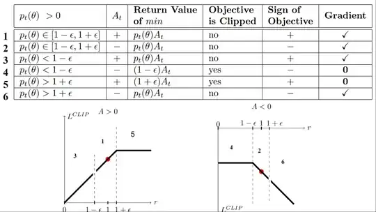
Case 1 and 2: the ratio is between the range

In situations 1 and 2, the clipping does not apply since the ratio is between the range $[1 - \epsilon, 1 + \epsilon]$

In situation 1, we have a positive advantage: the action is better than the average of all the actions in that state. Therefore, we should encourage our current policy to increase the probability of taking that action in that state.

Since the ratio is between intervals, we can increase our policy’s probability of taking that action at that state.

In situation 2, we have a negative advantage: the action is worse than the average of all actions at that state. Therefore, we should discourage our current policy from taking that action in that state.

Since the ratio is between intervals, ** the probability that our policy takes that action at that state**

Case 3 and 4: the ratio is below the range

If the probability ratio is lower than $[1 - \epsilon]$, the probability of taking that action at that state is much lower than with the old policy.

If, like in situation 3, the advantage estimate is positive ($A>0$), then you want to increase the probability of taking that action at that state.

But if, like situation 4, the advantage estimate is negative, we don’t want to decrease further the probability of taking that action at that state. Therefore, the gradient is = 0 (since we’re on a flat line), so we don’t update our weights.

Case 5 and 6: the ratio is above the range

If the probability ratio is higher than $[1 + \epsilon]$, the probability of taking that action at that state in the current policy is much higher than in the former policy.

If, like in situation 5, the advantage is positive, we don’t want to get too greedy. We already have a higher probability of taking that action at that state than the former policy. Therefore, the gradient is = 0 (since we’re on a flat line), so we don’t update our weights.

If, like in situation 6, the advantage is negative, we want to decrease the probability of taking that action at that state.

So if we recap, we only update the policy with the unclipped objective part. When the minimum is the clipped objective part, we don’t update our policy weights since the gradient will equal 0.

Source: DEEP RL Course - Visualize the Clipped Surrogate Objective Function

Deb
  • 101
  • 2